Veri yapıları
Veri tipleri
- Vektör: Bir boyutlu (sütunlu) veri (bir eleman da olabilir)
- Matriks: İki-boyutlu veri (bütün satır ve sütunlar aynı veri tipinde olmalı)
- Dizi (array): Çok boyutlu veri (bütün satır ve sütunlar aynı veri tipinde olmalı)
- Dataframe: Matrikse benzer, fakat sütünlarda farklı veri tipleri olabilir
- Dataframe R’da en çok kullanılan veri yapısıdır
- Datatable: Dataframe’e benzer fakat ek özellikleri var
- Liste: R’daki nesnelerin herhangi bir şekilde birleşimi
Dataframe
- Dataframe’in satır, sütun ve hücrelerine endeksleme ile erişilebilir
df <- data.frame(a = c(1,2,3,4,5), b=c(4, 3, 6, 1, 1), c=c("a", "a", "b", "c", "c"))
# A column
df[, 3]
## [1] "a" "a" "b" "c" "c"
df[,"c"]
## [1] "a" "a" "b" "c" "c"
df$c
## [1] "a" "a" "b" "c" "c"
# Single cell
df[2,3]
## [1] "a"
df$c[2]
## [1] "a"
# A row
df[2,]
##   a b c
## 2 2 3 a
# A range
df[3:5, 2:3]
##   b c
## 3 6 b
## 4 1 c
## 5 1 c
# By name
df[3:4, "c"]
## [1] "b" "c"
# İki dataframe'in birleştirilmesi
dc <- data.frame(d = c(10,20,30,40,50), e=c("a1", "a2", "b3", "d3", "e2"))
dr <- c(100,200,300,400, 500)
# Sürunların birleştirilmesi
df
##   a b c
## 1 1 4 a
## 2 2 3 a
## 3 3 6 b
## 4 4 1 c
## 5 5 1 c
df <- cbind(df, dc)
df
##   a b c  d  e
## 1 1 4 a 10 a1
## 2 2 3 a 20 a2
## 3 3 6 b 30 b3
## 4 4 1 c 40 d3
## 5 5 1 c 50 e2
# Satırların birleştirilmesi
df <- rbind(df, dr)
df
##     a   b   c   d   e
## 1   1   4   a  10  a1
## 2   2   3   a  20  a2
## 3   3   6   b  30  b3
## 4   4   1   c  40  d3
## 5   5   1   c  50  e2
## 6 100 200 300 400 500
# Kayıp değerlere dikkat!
Veri girişi
Klavyeden
dt <- data.frame(a = c(1:10), b = rnorm(10, 0, 0.5), c = c(1:2))
dt$d <- dt$a + dt$b + 2*dt$c
dt <- within(dt, e <- a + b + 2*c)
dt
##     a            b c         d         e
## 1   1 -0.110314183 1  2.889686  2.889686
## 2   2  0.737505690 2  6.737506  6.737506
## 3   3 -0.434922071 1  4.565078  4.565078
## 4   4  0.545903118 2  8.545903  8.545903
## 5   5  0.345337854 1  7.345338  7.345338
## 6   6  1.105701487 2 11.105701 11.105701
## 7   7 -0.295803538 1  8.704196  8.704196
## 8   8  0.102604390 2 12.102604 12.102604
## 9   9 -0.019823804 1 10.980176 10.980176
## 10 10 -0.002684118 2 13.997316 13.997316
a <- c(1, 2, 4, 2, 6, 3, 5, 8, 1, 10)
b <- rep(c(2:3), times=5)
c <- rep(c(2:3), each=5)
d <- rep(c(2:3), length.out=10)
e <- seq(0, 180, length.out = 10)
f <- seq(0, 45, by=5)
dd <- data.frame(a, b, c, d, e, f)
dd
##     a b c d   e  f
## 1   1 2 2 2   0  0
## 2   2 3 2 3  20  5
## 3   4 2 2 2  40 10
## 4   2 3 2 3  60 15
## 5   6 2 2 2  80 20
## 6   3 3 3 3 100 25
## 7   5 2 3 2 120 30
## 8   8 3 3 3 140 35
## 9   1 2 3 2 160 40
## 10 10 3 3 3 180 45
Boş data.frame
dt <- data.frame(a = character(), b = integer(), c = double())
dt
## [1] a b c
## <0 rows> (or 0-length row.names)
summary(dt)
##       a                   b             c
##  Length:0           Min.   : NA   Min.   : NA
##  Class :character   1st Qu.: NA   1st Qu.: NA
##  Mode  :character   Median : NA   Median : NA
##                     Mean   :NaN   Mean   :NaN
##                     3rd Qu.: NA   3rd Qu.: NA
##                     Max.   : NA   Max.   : NA
Veri setinin hazırlanması
Verilerin kontrolü
- RStudio “Environment” panosu
- Verilerin yapısı
dt <- data.frame(a = c(1:1000), b = rnorm(1000, 0, 1),
    c = c(1:2), d = sample(5, 1000, replace = TRUE))
dt$b[runif(100)<0.1] <- NA
dt$d[runif(100)<0.1] <- NA
dt <- within(dt, e <- c + (c-1)*d  + (b * (c-1) * (d/5)) + rnorm(1000, 0, 1))
head(dt)
##   a          b c d           e
## 1 1  1.4874246 1 2  0.64169858
## 2 2 -1.0508524 2 1  2.32425844
## 3 3  0.5817901 1 3  0.07467004
## 4 4 -0.5332055 2 2  3.64497847
## 5 5  0.2112661 1 5 -1.36033202
## 6 6  1.9089065 2 1  2.04316760
tail(dt)
##         a          b c d          e
## 995   995         NA 1 4         NA
## 996   996         NA 2 2         NA
## 997   997 -0.6026947 1 5 -0.4142646
## 998   998  1.5214073 2 1  3.5291314
## 999   999         NA 1 2         NA
## 1000 1000 -0.3858548 2 5  7.5122408
colnames(dt)
## [1] "a" "b" "c" "d" "e"
dim(dt)
## [1] 1000 5
str(dt)
## 'data.frame':    1000 obs. of  5 variables:
##  $ a: int  1 2 3 4 5 6 7 8 9 10 ...
##  $ b: num  1.487 -1.051 0.582 -0.533 0.211 ...
##  $ c: int  1 2 1 2 1 2 1 2 1 2 ...
##  $ d: int  2 1 3 2 5 1 1 2 3 NA ...
##  $ e: num  0.6417 2.3243 0.0747 3.645 -1.3603 ...
table(dt$d)
##
##   1   2   3   4   5
## 170 181 169 165 185
table(dt$c, dt$d)
##
##      1  2  3  4  5
##   1 85 97 84 87 87
##   2 85 84 85 78 98
xtabs( ~ c + d, data = dt)
##    d
## c    1  2  3  4  5
##   1 85 97 84 87 87
##   2 85 84 85 78 98
Kayıp değerler
library(mice)
##
## Attaching package: 'mice'
## The following object is masked from 'package:stats':
##
##     filter
## The following objects are masked from 'package:base':
##
##     cbind, rbind
# Kayıp değer yapısı
md.pattern(dt)

##     a c   d   b   e
## 720 1 1   1   1   1   0
## 150 1 1   1   0   0   2
## 130 1 1   0   1   0   2
##     0 0 130 150 280 560
Betimleyici istatistikler
summary(dt)
##        a                b                  c             d
##  Min.   :   1.0   Min.   :-3.29517   Min.   :1.0   Min.   :1.000
##  1st Qu.: 250.8   1st Qu.:-0.64958   1st Qu.:1.0   1st Qu.:2.000
##  Median : 500.5   Median : 0.01648   Median :1.5   Median :3.000
##  Mean   : 500.5   Mean   :-0.01181   Mean   :1.5   Mean   :3.016
##  3rd Qu.: 750.2   3rd Qu.: 0.63198   3rd Qu.:2.0   3rd Qu.:4.000
##  Max.   :1000.0   Max.   : 3.84948   Max.   :2.0   Max.   :5.000
##                   NA's   :150                      NA's   :130
##        e
##  Min.   :-1.9323
##  1st Qu.: 0.9438
##  Median : 2.4784
##  Mean   : 3.0462
##  3rd Qu.: 4.9936
##  Max.   :10.1617
##  NA's   :280
summary(subset(dt, c == 1))
##        a               b                  c           d
##  Min.   :  1.0   Min.   :-3.29517   Min.   :1   Min.   :1.000
##  1st Qu.:250.5   1st Qu.:-0.64983   1st Qu.:1   1st Qu.:2.000
##  Median :500.0   Median :-0.03122   Median :1   Median :3.000
##  Mean   :500.0   Mean   :-0.01182   Mean   :1   Mean   :2.986
##  3rd Qu.:749.5   3rd Qu.: 0.61848   3rd Qu.:1   3rd Qu.:4.000
##  Max.   :999.0   Max.   : 3.84948   Max.   :1   Max.   :5.000
##                  NA's   :100                    NA's   :60
##        e
##  Min.   :-1.9323
##  1st Qu.: 0.2003
##  Median : 0.9056
##  Mean   : 0.8877
##  3rd Qu.: 1.6223
##  Max.   : 2.9781
##  NA's   :160
summary(subset(dt, c == 2))
##        a                b                  c           d
##  Min.   :   2.0   Min.   :-3.16689   Min.   :2   Min.   :1.000
##  1st Qu.: 251.5   1st Qu.:-0.64912   1st Qu.:2   1st Qu.:2.000
##  Median : 501.0   Median : 0.03724   Median :2   Median :3.000
##  Mean   : 501.0   Mean   :-0.01180   Mean   :2   Mean   :3.047
##  3rd Qu.: 750.5   3rd Qu.: 0.64034   3rd Qu.:2   3rd Qu.:4.000
##  Max.   :1000.0   Max.   : 2.84511   Max.   :2   Max.   :5.000
##                   NA's   :50                     NA's   :70
##        e
##  Min.   : 0.7269
##  1st Qu.: 3.5539
##  Median : 4.8408
##  Mean   : 4.9775
##  3rd Qu.: 6.4397
##  Max.   :10.1617
##  NA's   :120
library(stargazer)
stargazer(dt, type="html", digits = 1)
|
|
|
Statistic
|
N
|
Mean
|
St. Dev.
|
Min
|
Pctl(25)
|
Pctl(75)
|
Max
|
|
|
|
a
|
1,000
|
500.5
|
288.8
|
1
|
250.8
|
750.2
|
1,000
|
|
b
|
850
|
-0.01
|
1.0
|
-3.3
|
-0.6
|
0.6
|
3.8
|
|
c
|
1,000
|
1.5
|
0.5
|
1
|
1
|
2
|
2
|
|
d
|
870
|
3.0
|
1.4
|
1.0
|
2.0
|
4.0
|
5.0
|
|
e
|
720
|
3.0
|
2.6
|
-1.9
|
0.9
|
5.0
|
10.2
|
|
|
Şekiller
library(ggplot2)
ggplot(dt, aes(x = b)) + geom_histogram()
## `stat_bin()` using `bins = 30`. Pick better value with `binwidth`.
## Warning: Removed 150 rows containing non-finite values (stat_bin).

ggplot(dt, aes(x = b)) + geom_density()
## Warning: Removed 150 rows containing non-finite values (stat_density).

ggplot(dt, aes(x = b)) + geom_density() +
 stat_function(fun = dnorm, args = list(mean = 0, sd = 1), col="blue")
## Warning: Removed 150 rows containing non-finite values (stat_density).

ggplot(dt, aes(x = d)) + geom_histogram()
## `stat_bin()` using `bins = 30`. Pick better value with `binwidth`.
## Warning: Removed 130 rows containing non-finite values (stat_bin).

ggplot(dt, aes(x = d)) + geom_histogram(binwidth=1)
## Warning: Removed 130 rows containing non-finite values (stat_bin).

ggplot(dt, aes(x = d)) + geom_bar()
## Warning: Removed 130 rows containing non-finite values (stat_count).

ggplot(dt, aes(x = d, y = b)) + geom_point()
## Warning: Removed 280 rows containing missing values (geom_point).

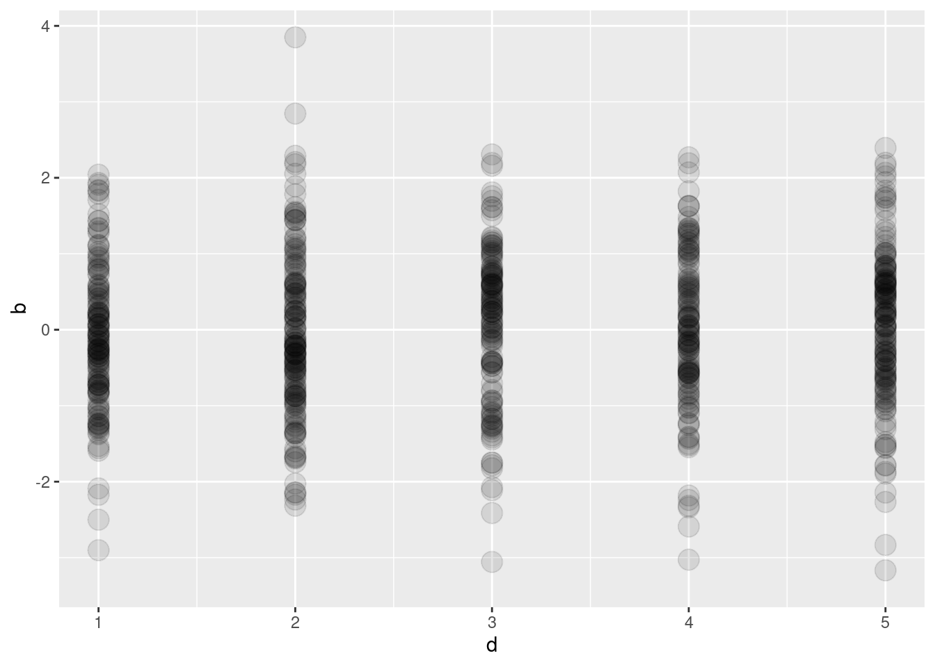
ggplot(dt, aes(x = d, y = b)) + geom_point(size=5, alpha=0.1)
## Warning: Removed 280 rows containing missing values (geom_point).
# Veriler üst üste geliyorsa...
ggplot(dt, aes(x = d, y = b)) + geom_jitter(size=5, alpha=0.5, width=0.5)
## Warning: Removed 280 rows containing missing values (geom_point).

# İki değişkenli şekiller
ggplot(dt, aes(x = b, y = e)) + geom_point()
## Warning: Removed 280 rows containing missing values (geom_point).

ggplot(dt, aes(x = b, y = e)) + geom_point() +
    geom_smooth(formula = y ~ x)
## `geom_smooth()` using method = 'gam'
## Warning: Removed 280 rows containing non-finite values (stat_smooth).

## Warning: Removed 280 rows containing missing values (geom_point).

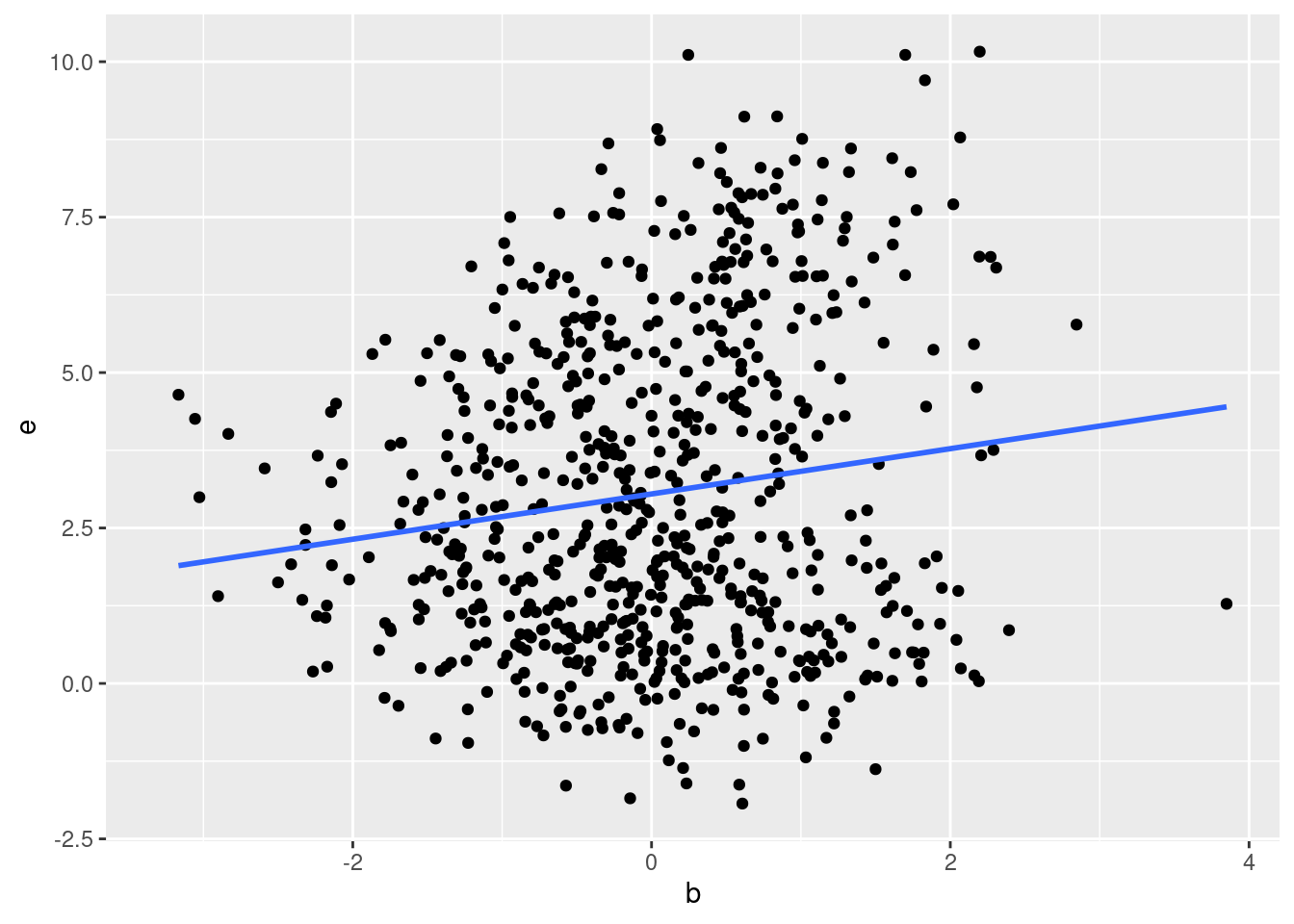
ggplot(dt, aes(x = b, y = e)) + geom_point() +
    geom_smooth(formula = y ~ x, se = FALSE, method = "lm")
## Warning: Removed 280 rows containing non-finite values (stat_smooth).

## Warning: Removed 280 rows containing missing values (geom_point).
ggplot(dt, aes(x = b, y = e)) + geom_point() + facet_wrap(~ c) +
    geom_smooth(formula = y ~ x, se = FALSE, method = "lm")
## Warning: Removed 280 rows containing non-finite values (stat_smooth).

## Warning: Removed 280 rows containing missing values (geom_point).

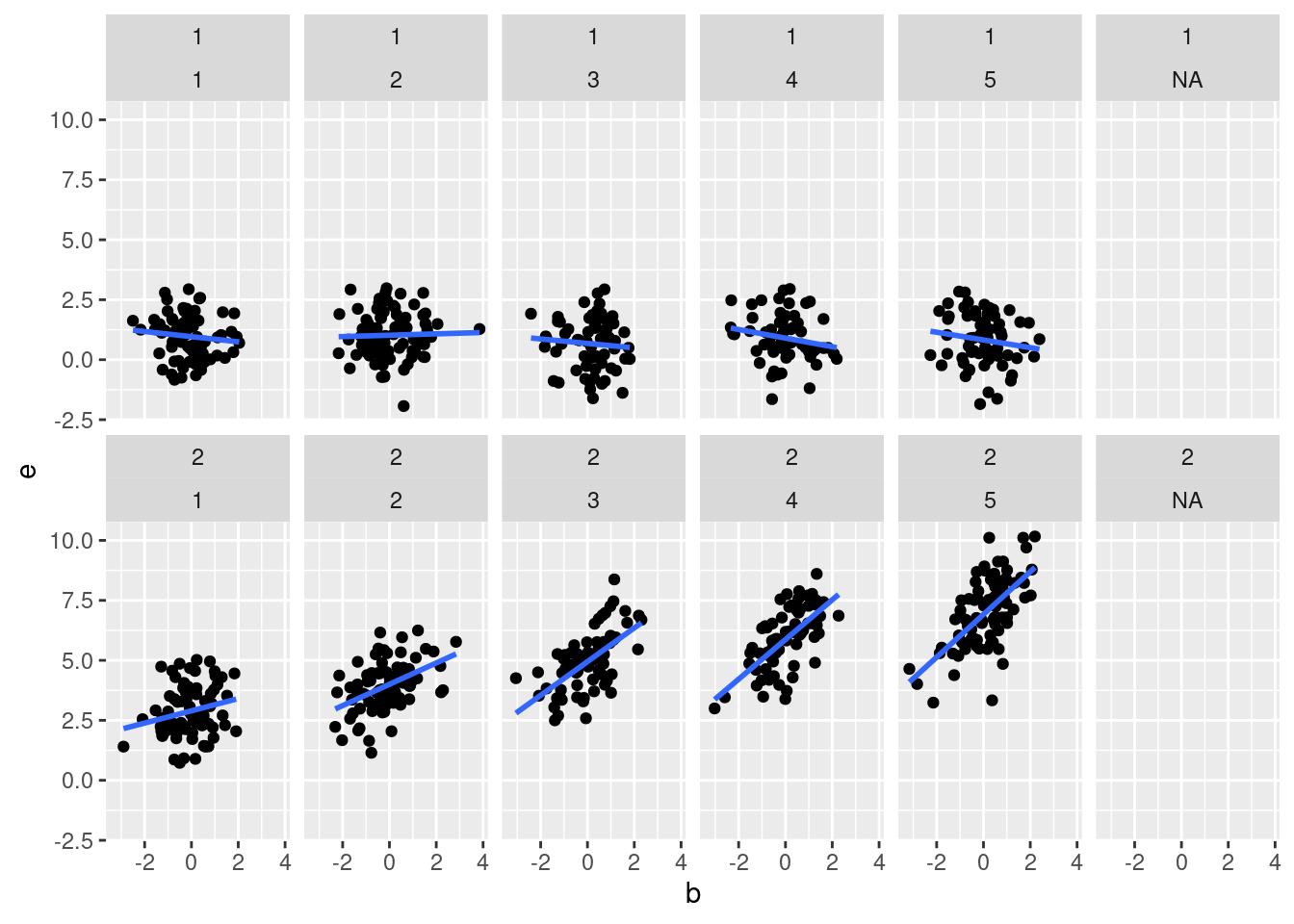
ggplot(dt, aes(x = b, y = e)) + geom_point() + facet_wrap(c ~ d, nrow = 2) +
    geom_smooth(formula = y ~ x, se = FALSE, method = "lm")
## Warning: Removed 280 rows containing non-finite values (stat_smooth).

## Warning: Removed 280 rows containing missing values (geom_point).
İlişkiler
# İlişkiler, 2-4. değişkenler
cor(dt[, 2:5])
##    b  c  d  e
## b  1 NA NA NA
## c NA  1 NA NA
## d NA NA  1 NA
## e NA NA NA  1
cor(dt[, 2:5], use = "complete.obs")
##             b           c          d         e
## b 1.000000000 0.003282638 0.05707731 0.1432851
## c 0.003282638 1.000000000 0.03461141 0.7942065
## d 0.057077311 0.034611407 1.00000000 0.3254381
## e 0.143285050 0.794206521 0.32543814 1.0000000
cor(dt[, 2:5], use = "pairwise.complete.obs")
##              b            c          d         e
## b 1.000000e+00 1.313176e-05 0.05707731 0.1432851
## c 1.313176e-05 1.000000e+00 0.02110836 0.7942065
## d 5.707731e-02 2.110836e-02 1.00000000 0.3254381
## e 1.432851e-01 7.942065e-01 0.32543814 1.0000000
cor(dt[, 2:5], use = "pairwise.complete.obs", method = "kendall")
##             b           c          d          e
## b 1.000000000 0.008805181 0.05463466 0.07277082
## c 0.008805181 1.000000000 0.01892767 0.67578456
## d 0.054634664 0.018927674 1.00000000 0.20302809
## e 0.072770824 0.675784563 0.20302809 1.00000000
cor(dt[, 2:5], use = "pairwise.complete.obs", method = "spearman")
##            b          c          d         e
## b 1.00000000 0.01077776 0.07668124 0.1057895
## c 0.01077776 1.00000000 0.02115924 0.8270895
## d 0.07668124 0.02115924 1.00000000 0.2591102
## e 0.10578952 0.82708951 0.25911024 1.0000000
Tüm değişkenler
- Tüm değişkenlere ait temel istatistiklerin tek komut ile gösterilmesi
library(GGally)
## Registered S3 method overwritten by 'GGally':
##   method from
##   +.gg   ggplot2
ggpairs(dt)

Temel testler
- Kategorik değişkenler için Chi-kare testi
tab <- xtabs(~ c + d, data = dt)
tab
##    d
## c    1  2  3  4  5
##   1 85 97 84 87 87
##   2 85 84 85 78 98
chisq.test(tab)
##
##  Pearson's Chi-squared test
##
## data:  tab
## X-squared = 1.9699, df = 4, p-value = 0.7413
- Sürekli değişkenler için t-testi
t.test(dt$b, mu = 0)
##
##  One Sample t-test
##
## data:  dt$b
## t = -0.34304, df = 849, p-value = 0.7317
## alternative hypothesis: true mean is not equal to 0
## 95 percent confidence interval:
##  -0.07938007  0.05576085
## sample estimates:
##   mean of x
## -0.01180961
t.test(dt$b, dt$e)
##
##  Welch Two Sample t-test
##
## data:  dt$b and dt$e
## t = -30.02, df = 903.64, p-value < 2.2e-16
## alternative hypothesis: true difference in means is not equal to 0
## 95 percent confidence interval:
##  -3.257928 -2.858081
## sample estimates:
##   mean of x   mean of y
## -0.01180961  3.04619514
t.test(dt$b, dt$e, var.equal = TRUE)
##
##  Two Sample t-test
##
## data:  dt$b and dt$e
## t = -31.909, df = 1568, p-value < 2.2e-16
## alternative hypothesis: true difference in means is not equal to 0
## 95 percent confidence interval:
##  -3.245983 -2.870027
## sample estimates:
##   mean of x   mean of y
## -0.01180961  3.04619514
with(dt, t.test(b[c == 1], b[c == 2]))
##
##  Welch Two Sample t-test
##
## data:  b[c == 1] and b[c == 2]
## t = -0.00038203, df = 832.94, p-value = 0.9997
## alternative hypothesis: true difference in means is not equal to 0
## 95 percent confidence interval:
##  -0.1356171  0.1355643
## sample estimates:
##   mean of x   mean of y
## -0.01182358 -0.01179719
Görselleştirme
Veri setini oluşturalım
library(ggplot2)
library(ggthemes)
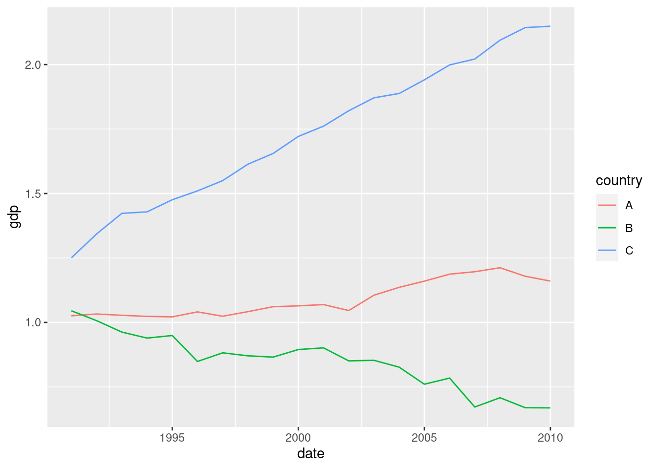
DT <- data.frame(country = rep(c("A", "B", "C"), each=20), date = rep(1991:2010, times=3),
    gdp = c(1 + cumsum(rnorm(20, 0.01, 0.02)), 1.1 + cumsum(rnorm(20, 0.01, 0.04)),
    1.2 + cumsum(rnorm(20, 0.04, 0.02))))
ggplot şekilleri
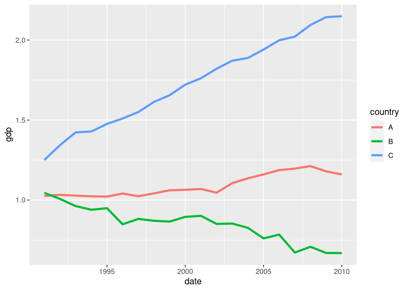
c1 <- ggplot(DT, aes(x=date, y=gdp, color=country)) + geom_line()
c1
# Daha kalın çizgiler
c1 <- ggplot(DT, aes(x=date, y=gdp, color=country)) + geom_line(size=1.25)
c1
# Sembol (legend) başlığının değiştirilmesi
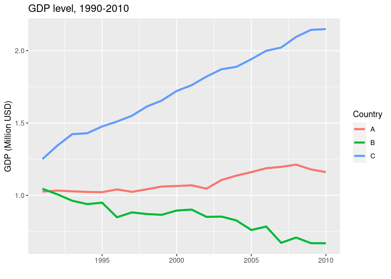
c1 <- c1 + guides(color = guide_legend(title = "Country"))
c1

# Başlıkların eklenmesi
c1 <- c1 + labs(title="GDP level, 1990-2010", x="", y="GDP (Million USD)")
c1
# HC teması
c1 + theme_hc()

# Economist teması
c1 + theme_economist()

Kişiselleştirilmiş tema
theme_et <- function (base_size = 12, base_family = "ubuntu") {
  theme(rect = element_rect(fill = "#FFFFFF", linetype = 0, colour = NA),
        text = element_text(size = base_size, family = base_family),
        plot.title = element_text( size = rel(1.1), hjust = 0.5),
        axis.title.x = element_text(hjust = 0.5, size = rel(0.85)),
        axis.title.y = element_text(hjust = 0.5, size = rel(0.85)),
        axis.text = element_text(colour = "black"),
        axis.line = element_line(colour = "black", size = rel(0.3)),
        legend.text = element_text(colour = "black", size= rel(.85)),
        panel.grid.major.y = element_line(color = "gray", size = rel(0.3)),
        panel.grid.major.x = element_blank(),
        panel.grid.minor.y = element_blank(), panel.grid.minor.x = element_blank(),
        panel.border = element_blank(), panel.background = element_blank(),
        legend.position = "bottom", legend.key = element_rect(fill = "#FFFFFF00"))
}

c1 + theme_et()

Temada değişiklik
c1 + theme(plot.title = element_text(size = rel(2), colour = "blue"))

c1 + theme(axis.text = element_text(colour = "blue", size=rel(1.5)))

c1 + theme(legend.position = "bottom")

c1 + theme(legend.position = c(0.5, 0.5))

c1 + theme(legend.position = "none")

c1 + theme(legend.text = element_text(size = 20, colour = "red", angle = 45))

# Metin eklenmesi
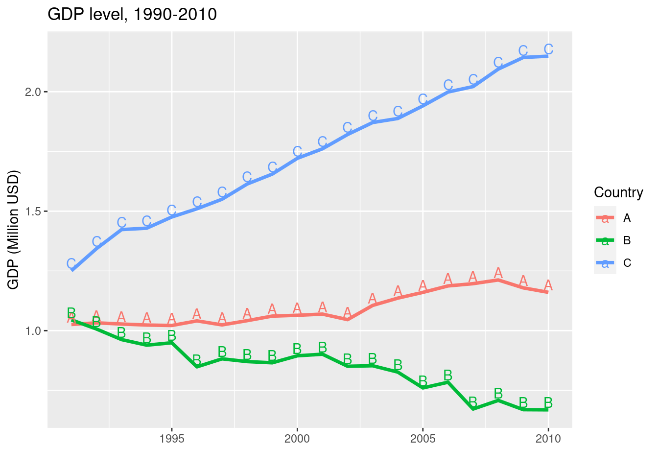
c1 + geom_text(data = DT, aes(x=date, y=gdp+.03, label = country))
# Formül eklenmesi
c1 + annotate("text", x=1995, y=1.5, parse=TRUE, label="frac(1, sqrt(2 * pi)) * e ^ {-x^2 / 2}")
