Create a dataset
- Load libraries to be used
library(data.table)
library(ggplot2)
library(mice)
##
## Attaching package: 'mice'
## The following object is masked from 'package:stats':
##
##     filter
## The following objects are masked from 'package:base':
##
##     cbind, rbind
library(plm)
##
## Attaching package: 'plm'
## The following object is masked from 'package:data.table':
##
##     between
library(stargazer)
##
## Please cite as:
## Hlavac, Marek (2018). stargazer: Well-Formatted Regression and Summary Statistics Tables.
## R package version 5.2.2. https://CRAN.R-project.org/package=stargazer
- Create a firm level dataset
nf <- 1000
nt <- 20
ns <- 10
nobs <- nf*nt

kelas <- 0.1
lelas <- 0.2
melas <- 0.75

id <- rep(c(1:nf), each = nt)
year <- rep(c(1:nt), times = nf)
sect <- rep(c(1:ns), each = nobs / ns)
kg <- rnorm(nobs, 0.01, 0.02)
lg <- (kg/10) + rnorm(nobs, 0.01, 0.01)
mg <- (lg/10) + rnorm(nobs, 0.005, 0.01)
tc <- rnorm(nobs, 0.01, 0.01)
fs <- max(0.1, rep(rnorm(nf, 2, 0.5), each = nt))
re <- max(0.1, rep(rnorm(nf, 0, 0.5), each = nt))
ee <- rnorm(nobs, 0, 0.1)

fdata <- data.table(id, year, sect, kg, lg, mg, tc, fs, re, ee)
fdata[, lk := fs*(1 + cumsum(kg)), by = id]
fdata[, ll := fs*(1 + cumsum(lg)), by = id]
fdata[, lm := fs*(1 + cumsum(mg)), by = id]
fdata[, lA := fs*(1 + cumsum(tc)), by = id]
fdata[, fe := max(0.1, rep(rnorm(nf, 0, 0.5)) + mean(lk)/5 + mean(ll)/5), by = id]
fdata[, lq := (lA + kelas*lk + lelas*ll + melas*lm) + ee]
fdata[, lqre := re + (lA + kelas*lk + lelas*ll + melas*lm) + ee]
fdata[, lqfe := fe + (lA + kelas*lk + lelas*ll + melas*lm) + ee]
- Add some missing values
- Generate purely random missing values, 2.5%
fdata[0.025 > runif(nf*nt), lk := NA]
fdata[0.025 > runif(nf*nt), ll := NA]
fdata[0.025 > runif(nf*nt), lm := NA]
- Generate missing values for all 2.5% of firms
fdata[id %in% sample(1:nf, floor(0.025*nf)), lk := NA]
fdata[id %in% sample(1:nf, floor(0.025*nf)), ll := NA]
fdata[id %in% sample(1:nf, floor(0.025*nf)), lm := NA]
Checking the dataset
head(fdata)
##    id year sect           kg            lg            mg          tc       fs
## 1:  1    1    1  0.038166224  0.0176786556  0.0121535882 0.010296893 3.519755
## 2:  1    2    1 -0.002389877  0.0008002707 -0.0050055960 0.006415697 3.519755
## 3:  1    3    1  0.015054000  0.0099916191 -0.0005462509 0.004894156 3.519755
## 4:  1    4    1  0.029267630 -0.0045586010 -0.0031849558 0.011625298 3.519755
## 5:  1    5    1  0.042247846  0.0365674853  0.0096194099 0.022825756 3.519755
## 6:  1    6    1 -0.006144479 -0.0027957013 -0.0106178658 0.013397397 3.519755
##          re           ee       lk       ll       lm       lA       fe       lq
## 1: 1.662997  0.029315386 3.654090 3.581979 3.562532 3.555997 3.117941 7.339017
## 2: 1.662997 -0.302349058 3.645679 3.584796 3.544914 3.578579 3.117941 7.016442
## 3: 1.662997  0.058755837 3.698665 3.619964 3.542991 3.595805 3.117941 7.405664
## 4: 1.662997  0.001972156 3.801680 3.603919 3.531781 3.636723 3.117941 7.388483
## 5: 1.662997  0.210709881 3.950382 3.732627 3.565639 3.717064 3.117941 7.743567
## 6: 1.662997 -0.057852495 3.928755 3.722787 3.528267 3.764220 3.117941 7.490000
##        lqre     lqfe
## 1: 9.002014 10.45696
## 2: 8.679439 10.13438
## 3: 9.068660 10.52361
## 4: 9.051480 10.50642
## 5: 9.406564 10.86151
## 6: 9.152997 10.60794
str(fdata)
## Classes 'data.table' and 'data.frame':   20000 obs. of  18 variables:
##  $ id  : int  1 1 1 1 1 1 1 1 1 1 ...
##  $ year: int  1 2 3 4 5 6 7 8 9 10 ...
##  $ sect: int  1 1 1 1 1 1 1 1 1 1 ...
##  $ kg  : num  0.03817 -0.00239 0.01505 0.02927 0.04225 ...
##  $ lg  : num  0.01768 0.0008 0.00999 -0.00456 0.03657 ...
##  $ mg  : num  0.012154 -0.005006 -0.000546 -0.003185 0.009619 ...
##  $ tc  : num  0.0103 0.00642 0.00489 0.01163 0.02283 ...
##  $ fs  : num  3.52 3.52 3.52 3.52 3.52 ...
##  $ re  : num  1.66 1.66 1.66 1.66 1.66 ...
##  $ ee  : num  0.02932 -0.30235 0.05876 0.00197 0.21071 ...
##  $ lk  : num  3.65 3.65 3.7 3.8 3.95 ...
##  $ ll  : num  3.58 3.58 3.62 3.6 3.73 ...
##  $ lm  : num  3.56 3.54 3.54 3.53 3.57 ...
##  $ lA  : num  3.56 3.58 3.6 3.64 3.72 ...
##  $ fe  : num  3.12 3.12 3.12 3.12 3.12 ...
##  $ lq  : num  7.34 7.02 7.41 7.39 7.74 ...
##  $ lqre: num  9 8.68 9.07 9.05 9.41 ...
##  $ lqfe: num  10.5 10.1 10.5 10.5 10.9 ...
##  - attr(*, ".internal.selfref")=<externalptr>
##  - attr(*, "index")= int(0)
##   ..- attr(*, "__id")= int(0)
summary(fdata)
##        id              year            sect            kg
##  Min.   :   1.0   Min.   : 1.00   Min.   : 1.0   Min.   :-0.06589
##  1st Qu.: 250.8   1st Qu.: 5.75   1st Qu.: 3.0   1st Qu.:-0.00341
##  Median : 500.5   Median :10.50   Median : 5.5   Median : 0.01015
##  Mean   : 500.5   Mean   :10.50   Mean   : 5.5   Mean   : 0.01012
##  3rd Qu.: 750.2   3rd Qu.:15.25   3rd Qu.: 8.0   3rd Qu.: 0.02359
##  Max.   :1000.0   Max.   :20.00   Max.   :10.0   Max.   : 0.09768
##
##        lg                  mg                   tc                 fs
##  Min.   :-0.029226   Min.   :-0.0327996   Min.   :-0.02979   Min.   :3.52
##  1st Qu.: 0.004154   1st Qu.:-0.0007273   1st Qu.: 0.00348   1st Qu.:3.52
##  Median : 0.011041   Median : 0.0060572   Median : 0.01012   Median :3.52
##  Mean   : 0.011038   Mean   : 0.0060593   Mean   : 0.01013   Mean   :3.52
##  3rd Qu.: 0.017917   3rd Qu.: 0.0128672   3rd Qu.: 0.01685   3rd Qu.:3.52
##  Max.   : 0.049368   Max.   : 0.0494958   Max.   : 0.05040   Max.   :3.52
##
##        re              ee                  lk              ll
##  Min.   :1.663   Min.   :-0.395939   Min.   :3.088   Min.   :3.424
##  1st Qu.:1.663   1st Qu.:-0.065688   1st Qu.:3.660   1st Qu.:3.722
##  Median :1.663   Median : 0.002009   Median :3.855   Median :3.915
##  Mean   :1.663   Mean   : 0.001445   Mean   :3.895   Mean   :3.932
##  3rd Qu.:1.663   3rd Qu.: 0.068890   3rd Qu.:4.093   3rd Qu.:4.123
##  Max.   :1.663   Max.   : 0.406620   Max.   :5.234   Max.   :4.838
##                                      NA's   :981     NA's   :953
##        lm              lA              fe              lq
##  Min.   :3.310   Min.   :3.382   Min.   :2.794   Min.   :6.952
##  1st Qu.:3.610   1st Qu.:3.703   1st Qu.:3.060   1st Qu.:7.556
##  Median :3.727   Median :3.881   Median :3.174   Median :7.863
##  Mean   :3.746   Mean   :3.897   Mean   :3.186   Mean   :7.884
##  3rd Qu.:3.858   3rd Qu.:4.070   3rd Qu.:3.282   3rd Qu.:8.188
##  Max.   :4.385   Max.   :4.851   Max.   :3.878   Max.   :9.194
##  NA's   :979
##       lqre             lqfe
##  Min.   : 8.615   Min.   : 9.888
##  1st Qu.: 9.219   1st Qu.:10.727
##  Median : 9.526   Median :11.054
##  Mean   : 9.547   Mean   :11.070
##  3rd Qu.: 9.851   3rd Qu.:11.387
##  Max.   :10.857   Max.   :12.714
##
table(fdata$year, fdata$sect)
##
##        1   2   3   4   5   6   7   8   9  10
##   1  100 100 100 100 100 100 100 100 100 100
##   2  100 100 100 100 100 100 100 100 100 100
##   3  100 100 100 100 100 100 100 100 100 100
##   4  100 100 100 100 100 100 100 100 100 100
##   5  100 100 100 100 100 100 100 100 100 100
##   6  100 100 100 100 100 100 100 100 100 100
##   7  100 100 100 100 100 100 100 100 100 100
##   8  100 100 100 100 100 100 100 100 100 100
##   9  100 100 100 100 100 100 100 100 100 100
##   10 100 100 100 100 100 100 100 100 100 100
##   11 100 100 100 100 100 100 100 100 100 100
##   12 100 100 100 100 100 100 100 100 100 100
##   13 100 100 100 100 100 100 100 100 100 100
##   14 100 100 100 100 100 100 100 100 100 100
##   15 100 100 100 100 100 100 100 100 100 100
##   16 100 100 100 100 100 100 100 100 100 100
##   17 100 100 100 100 100 100 100 100 100 100
##   18 100 100 100 100 100 100 100 100 100 100
##   19 100 100 100 100 100 100 100 100 100 100
##   20 100 100 100 100 100 100 100 100 100 100
table(fdata$year, fdata$sect)
##
##        1   2   3   4   5   6   7   8   9  10
##   1  100 100 100 100 100 100 100 100 100 100
##   2  100 100 100 100 100 100 100 100 100 100
##   3  100 100 100 100 100 100 100 100 100 100
##   4  100 100 100 100 100 100 100 100 100 100
##   5  100 100 100 100 100 100 100 100 100 100
##   6  100 100 100 100 100 100 100 100 100 100
##   7  100 100 100 100 100 100 100 100 100 100
##   8  100 100 100 100 100 100 100 100 100 100
##   9  100 100 100 100 100 100 100 100 100 100
##   10 100 100 100 100 100 100 100 100 100 100
##   11 100 100 100 100 100 100 100 100 100 100
##   12 100 100 100 100 100 100 100 100 100 100
##   13 100 100 100 100 100 100 100 100 100 100
##   14 100 100 100 100 100 100 100 100 100 100
##   15 100 100 100 100 100 100 100 100 100 100
##   16 100 100 100 100 100 100 100 100 100 100
##   17 100 100 100 100 100 100 100 100 100 100
##   18 100 100 100 100 100 100 100 100 100 100
##   19 100 100 100 100 100 100 100 100 100 100
##   20 100 100 100 100 100 100 100 100 100 100
# Check the pattern of missing data
md.pattern(fdata)

##       id year sect kg lg mg tc fs re ee lA fe lq lqre lqfe  ll  lm  lk
## 17224  1    1    1  1  1  1  1  1  1  1  1  1  1    1    1   1   1   1    0
## 914    1    1    1  1  1  1  1  1  1  1  1  1  1    1    1   1   1   0    1
## 872    1    1    1  1  1  1  1  1  1  1  1  1  1    1    1   1   0   1    1
## 37     1    1    1  1  1  1  1  1  1  1  1  1  1    1    1   1   0   0    2
## 854    1    1    1  1  1  1  1  1  1  1  1  1  1    1    1   0   1   1    1
## 29     1    1    1  1  1  1  1  1  1  1  1  1  1    1    1   0   1   0    2
## 69     1    1    1  1  1  1  1  1  1  1  1  1  1    1    1   0   0   1    2
## 1      1    1    1  1  1  1  1  1  1  1  1  1  1    1    1   0   0   0    3
##        0    0    0  0  0  0  0  0  0  0  0  0  0    0    0 953 979 981 2913
# Use a dataset with only non-missing data
cdata <- na.omit(fdata)
dim(fdata)
## [1] 20000 18
dim(cdata)
## [1] 17224 18
# List all tables in the dataset
tables()
##     NAME   NROW NCOL MB                      COLS KEY
## 1: cdata 17,224   18  2 id,year,sect,kg,lg,mg,...
## 2: fdata 20,000   18  3 id,year,sect,kg,lg,mg,...
## Total: 5MB
Datatable operations
- DT[ i, j, by ]
- Take DT
- subset rows using i,
- then calculate j
- grouped by by
Deleting variables
# One variable
fdata[, kg := NULL]
# Many variables
fdata[, c("lg", "mg", "tc", "fs", "fe", "ee") := NULL]
Subsetting rows
# Rows 3-5
fdata[3:5,]
##    id year sect       re       lk       ll       lm       lA       lq     lqre
## 1:  1    3    1 1.662997 3.698665 3.619964 3.542991 3.595805 7.405664 9.068660
## 2:  1    4    1 1.662997 3.801680 3.603919 3.531781 3.636723 7.388483 9.051480
## 3:  1    5    1 1.662997 3.950382 3.732627 3.565639 3.717064 7.743567 9.406564
##        lqfe
## 1: 10.52361
## 2: 10.50642
## 3: 10.86151
fdata[3:5]
##    id year sect       re       lk       ll       lm       lA       lq     lqre
## 1:  1    3    1 1.662997 3.698665 3.619964 3.542991 3.595805 7.405664 9.068660
## 2:  1    4    1 1.662997 3.801680 3.603919 3.531781 3.636723 7.388483 9.051480
## 3:  1    5    1 1.662997 3.950382 3.732627 3.565639 3.717064 7.743567 9.406564
##        lqfe
## 1: 10.52361
## 2: 10.50642
## 3: 10.86151
# All rows where id == 1
fdata[id == 1]
##     id year sect       re       lk       ll       lm       lA       lq     lqre
##  1:  1    1    1 1.662997 3.654090 3.581979 3.562532 3.555997 7.339017 9.002014
##  2:  1    2    1 1.662997 3.645679 3.584796 3.544914 3.578579 7.016442 8.679439
##  3:  1    3    1 1.662997 3.698665 3.619964 3.542991 3.595805 7.405664 9.068660
##  4:  1    4    1 1.662997 3.801680 3.603919 3.531781 3.636723 7.388483 9.051480
##  5:  1    5    1 1.662997 3.950382 3.732627 3.565639 3.717064 7.743567 9.406564
##  6:  1    6    1 1.662997 3.928755 3.722787 3.528267 3.764220 7.490000 9.152997
##  7:  1    7    1 1.662997 3.893305 3.768023 3.554715 3.822195 7.695845 9.358842
##  8:  1    8    1 1.662997 4.039126 3.826286 3.597252 3.843946 7.750134 9.413131
##  9:  1    9    1 1.662997 4.158214 3.876467 3.636825 3.842764 7.667407 9.330403
## 10:  1   10    1 1.662997 4.121004 3.886315 3.642354 3.855608 7.785582 9.448579
## 11:  1   11    1 1.662997 4.174844 3.918006 3.702501 3.921153 7.808018 9.471015
## 12:  1   12    1 1.662997 4.199842 3.965014 3.645970 3.980418 7.991236 9.654233
## 13:  1   13    1 1.662997 4.291241 4.021858 3.769333 3.990719 8.093572 9.756568
## 14:  1   14    1 1.662997 4.272546 4.039630 3.820753 4.022212 8.069116 9.732112
## 15:  1   15    1 1.662997 4.261133 4.055126       NA 4.078983 8.224219 9.887216
## 16:  1   16    1 1.662997 4.325982 4.065531 3.811969 4.064955 8.107242 9.770238
## 17:  1   17    1 1.662997 4.364061 4.102125 3.821589 4.057188 8.273419 9.936415
## 18:  1   18    1 1.662997 4.439149 4.150308 3.844582 4.120032 8.098494 9.761490
## 19:  1   19    1 1.662997 4.387757 4.170929 3.890568 4.153501 8.172021 9.835017
## 20:  1   20    1 1.662997       NA 4.193363 3.877766 4.170695 8.176897 9.839893
##         lqfe
##  1: 10.45696
##  2: 10.13438
##  3: 10.52361
##  4: 10.50642
##  5: 10.86151
##  6: 10.60794
##  7: 10.81379
##  8: 10.86808
##  9: 10.78535
## 10: 10.90352
## 11: 10.92596
## 12: 11.10918
## 13: 11.21151
## 14: 11.18706
## 15: 11.34216
## 16: 11.22518
## 17: 11.39136
## 18: 11.21644
## 19: 11.28996
## 20: 11.29484
setkey(fdata, id, year)
fdata[.(1)]
##     id year sect       re       lk       ll       lm       lA       lq     lqre
##  1:  1    1    1 1.662997 3.654090 3.581979 3.562532 3.555997 7.339017 9.002014
##  2:  1    2    1 1.662997 3.645679 3.584796 3.544914 3.578579 7.016442 8.679439
##  3:  1    3    1 1.662997 3.698665 3.619964 3.542991 3.595805 7.405664 9.068660
##  4:  1    4    1 1.662997 3.801680 3.603919 3.531781 3.636723 7.388483 9.051480
##  5:  1    5    1 1.662997 3.950382 3.732627 3.565639 3.717064 7.743567 9.406564
##  6:  1    6    1 1.662997 3.928755 3.722787 3.528267 3.764220 7.490000 9.152997
##  7:  1    7    1 1.662997 3.893305 3.768023 3.554715 3.822195 7.695845 9.358842
##  8:  1    8    1 1.662997 4.039126 3.826286 3.597252 3.843946 7.750134 9.413131
##  9:  1    9    1 1.662997 4.158214 3.876467 3.636825 3.842764 7.667407 9.330403
## 10:  1   10    1 1.662997 4.121004 3.886315 3.642354 3.855608 7.785582 9.448579
## 11:  1   11    1 1.662997 4.174844 3.918006 3.702501 3.921153 7.808018 9.471015
## 12:  1   12    1 1.662997 4.199842 3.965014 3.645970 3.980418 7.991236 9.654233
## 13:  1   13    1 1.662997 4.291241 4.021858 3.769333 3.990719 8.093572 9.756568
## 14:  1   14    1 1.662997 4.272546 4.039630 3.820753 4.022212 8.069116 9.732112
## 15:  1   15    1 1.662997 4.261133 4.055126       NA 4.078983 8.224219 9.887216
## 16:  1   16    1 1.662997 4.325982 4.065531 3.811969 4.064955 8.107242 9.770238
## 17:  1   17    1 1.662997 4.364061 4.102125 3.821589 4.057188 8.273419 9.936415
## 18:  1   18    1 1.662997 4.439149 4.150308 3.844582 4.120032 8.098494 9.761490
## 19:  1   19    1 1.662997 4.387757 4.170929 3.890568 4.153501 8.172021 9.835017
## 20:  1   20    1 1.662997       NA 4.193363 3.877766 4.170695 8.176897 9.839893
##         lqfe
##  1: 10.45696
##  2: 10.13438
##  3: 10.52361
##  4: 10.50642
##  5: 10.86151
##  6: 10.60794
##  7: 10.81379
##  8: 10.86808
##  9: 10.78535
## 10: 10.90352
## 11: 10.92596
## 12: 11.10918
## 13: 11.21151
## 14: 11.18706
## 15: 11.34216
## 16: 11.22518
## 17: 11.39136
## 18: 11.21644
## 19: 11.28996
## 20: 11.29484
fdata[.(c(1:2)), .(id, year, sect, lq)]
##     id year sect       lq
##  1:  1    1    1 7.339017
##  2:  1    2    1 7.016442
##  3:  1    3    1 7.405664
##  4:  1    4    1 7.388483
##  5:  1    5    1 7.743567
##  6:  1    6    1 7.490000
##  7:  1    7    1 7.695845
##  8:  1    8    1 7.750134
##  9:  1    9    1 7.667407
## 10:  1   10    1 7.785582
## 11:  1   11    1 7.808018
## 12:  1   12    1 7.991236
## 13:  1   13    1 8.093572
## 14:  1   14    1 8.069116
## 15:  1   15    1 8.224219
## 16:  1   16    1 8.107242
## 17:  1   17    1 8.273419
## 18:  1   18    1 8.098494
## 19:  1   19    1 8.172021
## 20:  1   20    1 8.176897
## 21:  2    1    1 7.217165
## 22:  2    2    1 7.339393
## 23:  2    3    1 7.720350
## 24:  2    4    1 7.396201
## 25:  2    5    1 7.345134
## 26:  2    6    1 7.568926
## 27:  2    7    1 7.525900
## 28:  2    8    1 7.338753
## 29:  2    9    1 7.780740
## 30:  2   10    1 7.671478
## 31:  2   11    1 7.699673
## 32:  2   12    1 7.857096
## 33:  2   13    1 7.847248
## 34:  2   14    1 8.113233
## 35:  2   15    1 8.171282
## 36:  2   16    1 8.277005
## 37:  2   17    1 8.429589
## 38:  2   18    1 8.388729
## 39:  2   19    1 8.286276
## 40:  2   20    1 8.254107
##     id year sect       lq
fdata[.(c(1:2), c(10,20))]
##    id year sect       re       lk       ll       lm       lA       lq     lqre
## 1:  1   10    1 1.662997 4.121004 3.886315 3.642354 3.855608 7.785582 9.448579
## 2:  2   20    1 1.662997 3.853523 4.432852 3.897073 4.238855 8.254107 9.917103
##        lqfe
## 1: 10.90352
## 2: 11.31052
fdata[(id %in% c(1,2)) & (year %in% c(10, 20))]
##    id year sect       re       lk       ll       lm       lA       lq     lqre
## 1:  1   10    1 1.662997 4.121004 3.886315 3.642354 3.855608 7.785582 9.448579
## 2:  1   20    1 1.662997       NA 4.193363 3.877766 4.170695 8.176897 9.839893
## 3:  2   10    1 1.662997       NA 4.079789 3.766919 3.703680 7.671478 9.334475
## 4:  2   20    1 1.662997 3.853523 4.432852 3.897073 4.238855 8.254107 9.917103
##        lqfe
## 1: 10.90352
## 2: 11.29484
## 3: 10.72789
## 4: 11.31052
fdata[.(c(1:2))][year %in% c(10, 20)]
##    id year sect       re       lk       ll       lm       lA       lq     lqre
## 1:  1   10    1 1.662997 4.121004 3.886315 3.642354 3.855608 7.785582 9.448579
## 2:  1   20    1 1.662997       NA 4.193363 3.877766 4.170695 8.176897 9.839893
## 3:  2   10    1 1.662997       NA 4.079789 3.766919 3.703680 7.671478 9.334475
## 4:  2   20    1 1.662997 3.853523 4.432852 3.897073 4.238855 8.254107 9.917103
##        lqfe
## 1: 10.90352
## 2: 11.29484
## 3: 10.72789
## 4: 11.31052
sM <- data.table(id=c(1,1,2,2), year=c(10,20,10,20))
sM
##    id year
## 1:  1   10
## 2:  1   20
## 3:  2   10
## 4:  2   20
fdata[sM]
##    id year sect       re       lk       ll       lm       lA       lq     lqre
## 1:  1   10    1 1.662997 4.121004 3.886315 3.642354 3.855608 7.785582 9.448579
## 2:  1   20    1 1.662997       NA 4.193363 3.877766 4.170695 8.176897 9.839893
## 3:  2   10    1 1.662997       NA 4.079789 3.766919 3.703680 7.671478 9.334475
## 4:  2   20    1 1.662997 3.853523 4.432852 3.897073 4.238855 8.254107 9.917103
##        lqfe
## 1: 10.90352
## 2: 11.29484
## 3: 10.72789
## 4: 11.31052
Selecting columns
# Rows 3-5 of column id
fdata[3:5, id]
## [1] 1 1 1
# Rows 3-5 of columns id, year and lq
fdata[3:5, .(id, year, lq)]
##    id year       lq
## 1:  1    3 7.405664
## 2:  1    4 7.388483
## 3:  1    5 7.743567
# NOTE: .() means list()

# First 10 rows of id, year, lq and lk for missing lk's
fdata[is.na(lk), .(id, year, lq, lk)][1:10]
##     id year       lq lk
##  1:  1   20 8.176897 NA
##  2:  2   10 7.671478 NA
##  3:  2   18 8.388729 NA
##  4:  4    5 7.647795 NA
##  5:  5    1 7.255430 NA
##  6:  5    6 7.872916 NA
##  7:  5    9 8.163708 NA
##  8:  9   19 8.627078 NA
##  9: 11    2 7.335539 NA
## 10: 15    4 7.481647 NA
# Mean of lq
fdata[, mean(lq)]
## [1] 7.88367
# Mean and standard deviation of lq
fdata[, .(mean(lq), sd(lq))]
##         V1        V2
## 1: 7.88367 0.4046326
# Mean and standard deviation of lk
fdata[, .(mean(lk), sd(lk))]
##    V1 V2
## 1: NA NA
# Assigning names to computed columns
fdata[, .(mean.lq = mean(lq), sd.lq = sd(lq))]
##    mean.lq     sd.lq
## 1: 7.88367 0.4046326
# Even functions can be written
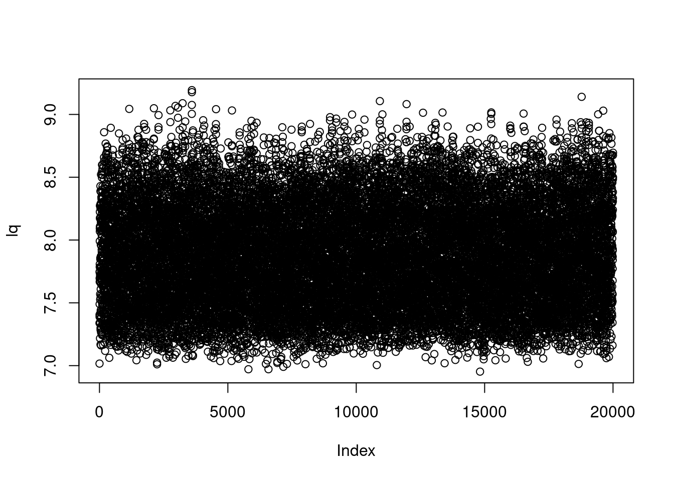
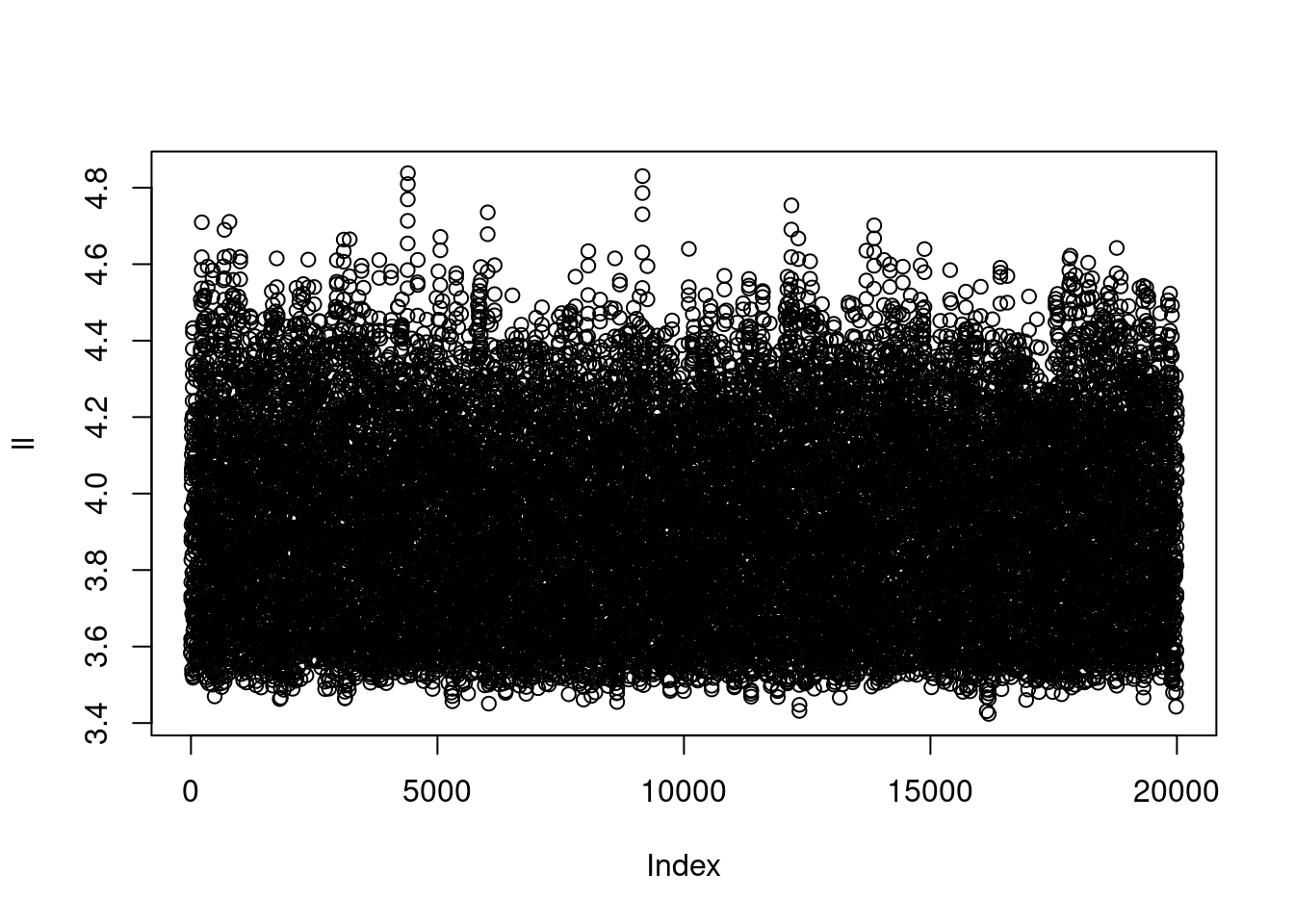
fdata[, {plot(lq)
        plot(ll)}]
## NULL
Rows and columns
# Doing __j__ by group
fdata[, .(mean.lq = mean(lq), sd.lq = sd(lq)), by=sect]
##     sect  mean.lq     sd.lq
##  1:    1 7.882924 0.4028988
##  2:    2 7.887971 0.4193219
##  3:    3 7.879297 0.4005734
##  4:    4 7.854285 0.3998991
##  5:    5 7.883481 0.4051014
##  6:    6 7.882825 0.3994798
##  7:    7 7.902018 0.4111187
##  8:    8 7.871442 0.3903540
##  9:    9 7.869953 0.3981443
## 10:   10 7.922500 0.4156736
# Doing __j__ by several groups
sectq <- fdata[, .(mean.lq = mean(lq), sd.lq = sd(lq)), by=.(sect, year)]
sectq
##      sect year  mean.lq     sd.lq
##   1:    1    1 7.280941 0.1033195
##   2:    1    2 7.339261 0.1096977
##   3:    1    3 7.411842 0.1275536
##   4:    1    4 7.468791 0.1257501
##   5:    1    5 7.557408 0.1400175
##  ---
## 196:   10   16 8.267393 0.2520468
## 197:   10   17 8.342998 0.2330403
## 198:   10   18 8.405878 0.2437114
## 199:   10   19 8.460349 0.2402204
## 200:   10   20 8.513158 0.2396596
tables()
##     NAME   NROW NCOL MB                      COLS     KEY
## 1: cdata 17,224   18  2 id,year,sect,kg,lg,mg,...
## 2: fdata 20,000   11  1 id,year,sect,re,lk,ll,... id,year
## 3: sectq    200    4  0   sect,year,mean.lq,sd.lq
## 4:    sM      4    2  0                   id,year
## Total: 3MB
# Call functions in by
fdata[, .(mean.lq = mean(lq), sd.lq = sd(lq)), by=.(sect, year>5)]
##     sect  year  mean.lq     sd.lq
##  1:    1 FALSE 7.411649 0.1553895
##  2:    1  TRUE 8.040016 0.3311458
##  3:    2 FALSE 7.399490 0.1576263
##  4:    2  TRUE 8.050799 0.3465371
##  5:    3 FALSE 7.404642 0.1585005
##  6:    3  TRUE 8.037516 0.3246832
##  7:    4 FALSE 7.389693 0.1486902
##  8:    4  TRUE 8.009148 0.3315212
##  9:    5 FALSE 7.409835 0.1583429
## 10:    5  TRUE 8.041363 0.3327555
## 11:    6 FALSE 7.416797 0.1476646
## 12:    6  TRUE 8.038167 0.3301001
## 13:    7 FALSE 7.415592 0.1442019
## 14:    7  TRUE 8.064160 0.3365168
## 15:    8 FALSE 7.411746 0.1574763
## 16:    8  TRUE 8.024674 0.3177482
## 17:    9 FALSE 7.410869 0.1516742
## 18:    9  TRUE 8.022981 0.3316665
## 19:   10 FALSE 7.437744 0.1622896
## 20:   10  TRUE 8.084086 0.3422591
fdata[, .(mean.lq = mean(lq), sd.lq = sd(lq), nobs = length(lq)), by=is.na(ll)]
##    is.na  mean.lq     sd.lq  nobs
## 1: FALSE 7.884207 0.4046362 19047
## 2:  TRUE 7.872937 0.4046219   953
# Grouping only on a subset
fdata[1:5, .(mean.lq = mean(lq), sd.lq = sd(lq)), by=.(year)]
##    year  mean.lq sd.lq
## 1:    1 7.339017    NA
## 2:    2 7.016442    NA
## 3:    3 7.405664    NA
## 4:    4 7.388483    NA
## 5:    5 7.743567    NA
# Using .N to get the total number of observations
fdata[is.na(lk), .N, by = sect]
##     sect   N
##  1:    1 139
##  2:    2 145
##  3:    3  86
##  4:    4  91
##  5:    5 128
##  6:    6  80
##  7:    7  93
##  8:    8  64
##  9:    9 103
## 10:   10  52
Creating/updating columns
head(fdata)
##    id year sect       re       lk       ll       lm       lA       lq     lqre
## 1:  1    1    1 1.662997 3.654090 3.581979 3.562532 3.555997 7.339017 9.002014
## 2:  1    2    1 1.662997 3.645679 3.584796 3.544914 3.578579 7.016442 8.679439
## 3:  1    3    1 1.662997 3.698665 3.619964 3.542991 3.595805 7.405664 9.068660
## 4:  1    4    1 1.662997 3.801680 3.603919 3.531781 3.636723 7.388483 9.051480
## 5:  1    5    1 1.662997 3.950382 3.732627 3.565639 3.717064 7.743567 9.406564
## 6:  1    6    1 1.662997 3.928755 3.722787 3.528267 3.764220 7.490000 9.152997
##        lqfe
## 1: 10.45696
## 2: 10.13438
## 3: 10.52361
## 4: 10.50642
## 5: 10.86151
## 6: 10.60794
fdata[, Q1 := exp(lq)]
head(fdata)
##    id year sect       re       lk       ll       lm       lA       lq     lqre
## 1:  1    1    1 1.662997 3.654090 3.581979 3.562532 3.555997 7.339017 9.002014
## 2:  1    2    1 1.662997 3.645679 3.584796 3.544914 3.578579 7.016442 8.679439
## 3:  1    3    1 1.662997 3.698665 3.619964 3.542991 3.595805 7.405664 9.068660
## 4:  1    4    1 1.662997 3.801680 3.603919 3.531781 3.636723 7.388483 9.051480
## 5:  1    5    1 1.662997 3.950382 3.732627 3.565639 3.717064 7.743567 9.406564
## 6:  1    6    1 1.662997 3.928755 3.722787 3.528267 3.764220 7.490000 9.152997
##        lqfe       Q1
## 1: 10.45696 1539.198
## 2: 10.13438 1114.813
## 3: 10.52361 1645.276
## 4: 10.50642 1617.251
## 5: 10.86151 2306.686
## 6: 10.60794 1790.053
# Be careful: DT <- DT[...] is redundant. The variables are added into DT
fdata[, c("K", "L", "M") := list(exp(lk), exp(ll), exp(lm))]
head(fdata)
##    id year sect       re       lk       ll       lm       lA       lq     lqre
## 1:  1    1    1 1.662997 3.654090 3.581979 3.562532 3.555997 7.339017 9.002014
## 2:  1    2    1 1.662997 3.645679 3.584796 3.544914 3.578579 7.016442 8.679439
## 3:  1    3    1 1.662997 3.698665 3.619964 3.542991 3.595805 7.405664 9.068660
## 4:  1    4    1 1.662997 3.801680 3.603919 3.531781 3.636723 7.388483 9.051480
## 5:  1    5    1 1.662997 3.950382 3.732627 3.565639 3.717064 7.743567 9.406564
## 6:  1    6    1 1.662997 3.928755 3.722787 3.528267 3.764220 7.490000 9.152997
##        lqfe       Q1        K        L        M
## 1: 10.45696 1539.198 38.63237 35.94461 35.25236
## 2: 10.13438 1114.813 38.30876 36.04600 34.63670
## 3: 10.52361 1645.276 40.39335 37.33622 34.57017
## 4: 10.50642 1617.251 44.77634 36.74194 34.18479
## 5: 10.86151 2306.686 51.95521 41.78876 35.36204
## 6: 10.60794 1790.053 50.84363 41.37957 34.06487
Indexing and keys
setkey(fdata, id, year)
fdata[.(1), .(id, year, Q1)]
##     id year       Q1
##  1:  1    1 1539.198
##  2:  1    2 1114.813
##  3:  1    3 1645.276
##  4:  1    4 1617.251
##  5:  1    5 2306.686
##  6:  1    6 1790.053
##  7:  1    7 2199.191
##  8:  1    8 2321.884
##  9:  1    9 2137.531
## 10:  1   10 2405.666
## 11:  1   11 2460.249
## 12:  1   12 2954.947
## 13:  1   13 3273.358
## 14:  1   14 3194.276
## 15:  1   15 3730.209
## 16:  1   16 3318.412
## 17:  1   17 3918.321
## 18:  1   18 3289.509
## 19:  1   19 3540.491
## 20:  1   20 3557.796
fdata[.(c(1:10)), mult = "first", .(id, year, Q1)]
##     id year       Q1
##  1:  1    1 1539.198
##  2:  2    1 1362.621
##  3:  3    1 1296.678
##  4:  4    1 1287.724
##  5:  5    1 1415.771
##  6:  6    1 1398.516
##  7:  7    1 1525.523
##  8:  8    1 1295.001
##  9:  9    1 1493.170
## 10: 10    1 1666.668
fdata[.(c(1:10)), mult = "last", .(id, year, Q1)]
##     id year       Q1
##  1:  1   20 3557.796
##  2:  2   20 3843.376
##  3:  3   20 5021.885
##  4:  4   20 4197.029
##  5:  5   20 5141.295
##  6:  6   20 5005.761
##  7:  7   20 4045.888
##  8:  8   20 3634.186
##  9:  9   20 7032.612
## 10: 10   20 4298.108
fdata[.(1,20)]
##    id year sect       re lk       ll       lm       lA       lq     lqre
## 1:  1   20    1 1.662997 NA 4.193363 3.877766 4.170695 8.176897 9.839893
##        lqfe       Q1  K        L        M
## 1: 11.29484 3557.796 NA 66.24517 48.31615
fdata[.(c(1:10)), sum(Q1), by = .EACHI]
##     id       V1
##  1:  1 52315.12
##  2:  2 53155.38
##  3:  3 51112.68
##  4:  4 53273.00
##  5:  5 68193.57
##  6:  6 59136.00
##  7:  7 56883.65
##  8:  8 56541.02
##  9:  9 68377.47
## 10: 10 55095.62
Changing variable names
setnames(fdata, "Q1", "Q")
# Changing variable names
fdata[, list(sum(Q), round(sum(L, na.rm = TRUE), 0)), by = year]
##     year      V1    V2
##  1:    1 1472008 33518
##  2:    2 1554934 35042
##  3:    3 1669885 36203
##  4:    4 1776699 37903
##  5:    5 1895561 39755
##  6:    6 2023243 41140
##  7:    7 2157393 42665
##  8:    8 2303066 44086
##  9:    9 2463944 46056
## 10:   10 2610844 48112
## 11:   11 2805176 50028
## 12:   12 2966837 51725
## 13:   13 3173448 54435
## 14:   14 3367423 56001
## 15:   15 3590105 58399
## 16:   16 3840746 61241
## 17:   17 4101192 63876
## 18:   18 4364959 65520
## 19:   19 4620901 67828
## 20:   20 4923453 70601
# Sorting
fdata[order(-year)]
##          id year sect       re       lk       ll       lm       lA       lq
##     1:    1   20    1 1.662997       NA 4.193363 3.877766 4.170695 8.176897
##     2:    2   20    1 1.662997 3.853523 4.432852 3.897073 4.238855 8.254107
##     3:    3   20    1 1.662997 3.876323 4.198807 3.923975 4.374655 8.521561
##     4:    4   20    1 1.662997 3.490346 4.076838 3.898902 4.318152 8.342132
##     5:    5   20    1 1.662997 4.794586 4.336500 3.750265 4.413677 8.545060
##    ---
## 19996:  996    1   10 1.662997 3.609362 3.551500 3.563476 3.509351 7.207576
## 19997:  997    1   10 1.662997 3.468721 3.479704 3.557001 3.569671 7.408829
## 19998:  998    1   10 1.662997 3.662068 3.567245 3.592026 3.590253 7.231715
## 19999:  999    1   10 1.662997 3.481653 3.620309 3.574346 3.552653 7.413591
## 20000: 1000    1   10 1.662997 3.556794 3.502435 3.540862 3.596059 7.161688
##             lqre     lqfe        Q         K        L        M
##     1:  9.839893 11.29484 3557.796        NA 66.24517 48.31615
##     2:  9.917103 11.31052 3843.376  47.15890 84.17110 49.25806
##     3: 10.184557 12.06827 5021.885  48.24647 66.60684 50.60120
##     4: 10.005129 11.34104 4197.029  32.79731 58.95877 49.34824
##     5: 10.208057 11.88587 5141.295 120.85433 76.43955 42.53233
##    ---
## 19996:  8.870573 10.26570 1349.617  36.94246 34.86557 35.28564
## 19997:  9.071825 10.74858 1650.492  32.09565 32.45010 35.05790
## 19998:  8.894712 10.80497 1382.592  38.94177 35.41887 36.30755
## 19999:  9.076588 10.59161 1658.371  32.51343 37.34912 35.67128
## 20000:  8.824685 10.19160 1289.085  35.05063 33.19618 34.49666
Chaining
fdata[, list(sum(Q), round(sum(L, na.rm = TRUE), 0)), by = year][order(-year)]
##     year      V1    V2
##  1:   20 4923453 70601
##  2:   19 4620901 67828
##  3:   18 4364959 65520
##  4:   17 4101192 63876
##  5:   16 3840746 61241
##  6:   15 3590105 58399
##  7:   14 3367423 56001
##  8:   13 3173448 54435
##  9:   12 2966837 51725
## 10:   11 2805176 50028
## 11:   10 2610844 48112
## 12:    9 2463944 46056
## 13:    8 2303066 44086
## 14:    7 2157393 42665
## 15:    6 2023243 41140
## 16:    5 1895561 39755
## 17:    4 1776699 37903
## 18:    3 1669885 36203
## 19:    2 1554934 35042
## 20:    1 1472008 33518
Melting and casting
- Melting: Transforming the dataset into long format
- Casting: Transforming the dataset into wide format
# Sectoral prices
sPrice <- data.table(
    year = c(1:nt),
    p1 = 1 + cumsum(rnorm(nt, 0.02, 0.04)),
    p2 = 1 + cumsum(rnorm(nt, 0.03, 0.05)),
    p3 = 1 + cumsum(rnorm(nt, 0.04, 0.02)),
    p4 = 1 + cumsum(rnorm(nt, 0.05, 0.03)),
    p5 = 1 + cumsum(rnorm(nt, 0.02, 0.04)),
    p6 = 1 + cumsum(rnorm(nt, 0.03, 0.06)),
    p7 = 1 + cumsum(rnorm(nt, 0.04, 0.02)),
    p8 = 1 + cumsum(rnorm(nt, 0.05, 0.07)),
    p9 = 1 + cumsum(rnorm(nt, 0.05, 0.04)),
    p10 = 1 + cumsum(rnorm(nt, 0.05, 0.06)))

head(sPrice)
##    year       p1        p2       p3       p4       p5       p6       p7
## 1:    1 1.108232 0.9725532 1.027199 1.038992 1.036930 1.085904 1.026963
## 2:    2 1.176799 1.0111537 1.087797 1.067987 1.073751 1.087087 1.073138
## 3:    3 1.224622 1.0144737 1.117243 1.095925 1.122481 1.216946 1.123270
## 4:    4 1.325986 1.0473948 1.207719 1.125843 1.149562 1.321952 1.174897
## 5:    5 1.339608 1.1176873 1.236809 1.199555 1.126223 1.435343 1.226882
## 6:    6 1.388677 1.1293030 1.324701 1.228623 1.183818 1.473882 1.275482
##           p8       p9      p10
## 1: 0.9697231 1.059323 1.082111
## 2: 0.9346809 1.142848 1.263425
## 3: 0.9488694 1.276297 1.350190
## 4: 1.0216512 1.278849 1.467613
## 5: 1.0332747 1.311174 1.621530
## 6: 1.1102063 1.361308 1.600860
sPriceM <- melt(sPrice, id.vars=1, variable.name = "sectName", value.name = "price")
head(sPriceM)
##    year sectName    price
## 1:    1       p1 1.108232
## 2:    2       p1 1.176799
## 3:    3       p1 1.224622
## 4:    4       p1 1.325986
## 5:    5       p1 1.339608
## 6:    6       p1 1.388677
sPriceM$sect <- as.numeric(unlist(gsub("[^0-9]", "", unlist(sPriceM$sectName)), ""))
sPriceM[, sectName := NULL]
head(sPriceM)
##    year    price sect
## 1:    1 1.108232    1
## 2:    2 1.176799    1
## 3:    3 1.224622    1
## 4:    4 1.325986    1
## 5:    5 1.339608    1
## 6:    6 1.388677    1
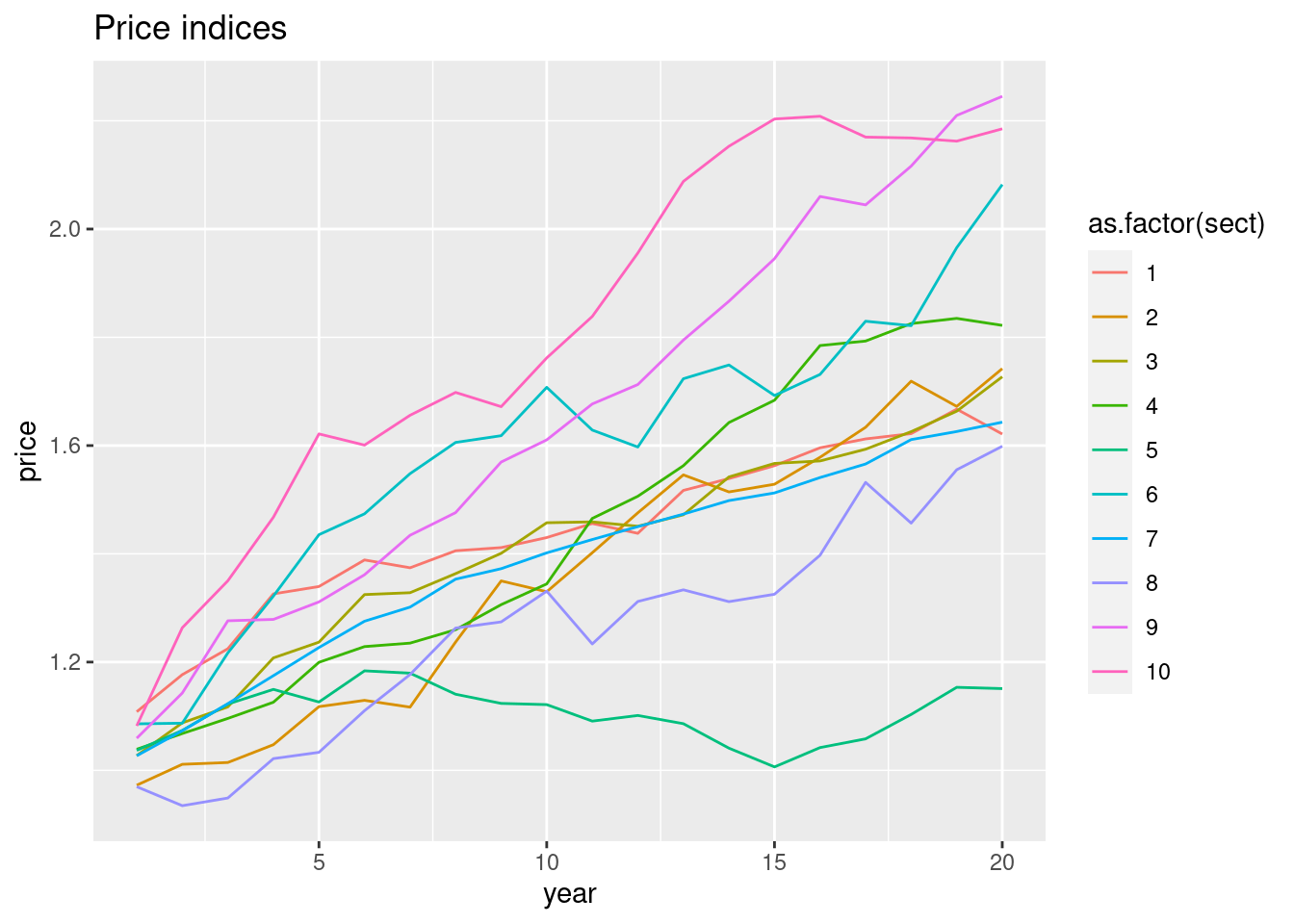
ggplot(sPriceM, aes(x=year, y=price, group=sect, color=as.factor(sect))) + geom_line() +
    ggtitle("Price indices")
setkey(sPriceM, sect, year)
setkey(fdata, sect, year)
fdataM <- fdata[sPriceM]
head(fdataM)
##    id year sect       re       lk       ll       lm       lA       lq     lqre
## 1:  1    1    1 1.662997 3.654090 3.581979 3.562532 3.555997 7.339017 9.002014
## 2:  2    1    1 1.662997 3.592924 3.539547 3.548782 3.545794 7.217165 8.880162
## 3:  3    1    1 1.662997 3.645341 3.518363 3.515378 3.573892 7.167561 8.830558
## 4:  4    1    1 1.662997 3.486291 3.610781 3.529788 3.542156 7.160632 8.823628
## 5:  5    1    1 1.662997       NA 3.551086 3.552183 3.608832 7.255430 8.918426
## 6:  6    1    1 1.662997 3.692298 3.531901 3.545200 3.575526 7.243167 8.906164
##        lqfe        Q        K        L        M    price
## 1: 10.45696 1539.198 38.63237 35.94461 35.25236 1.108232
## 2: 10.27358 1362.621 36.34020 34.45132 34.77095 1.108232
## 3: 10.71427 1296.678 38.29582 33.72916 33.62864 1.108232
## 4: 10.15954 1287.724 32.66456 36.99495 34.11673 1.108232
## 5: 10.59623 1415.771       NA 34.85115 34.88941 1.108232
## 6: 10.26458 1398.516 40.13699 34.18889 34.64663 1.108232
Merging datasets
- Create sector level variables
sdata <- fdata[, .(sQ = sum(Q, na.rm=T), sL = sum(L, na.rm=T), sM = sum(M, na.rm=T)),
    by = .(sect, year)]
summary(sdata)
##       sect           year             sQ               sL             sM
##  Min.   : 1.0   Min.   : 1.00   Min.   :144307   Min.   :3275   Min.   :3153
##  1st Qu.: 3.0   1st Qu.: 5.75   1st Qu.:197497   1st Qu.:4043   1st Qu.:3611
##  Median : 5.5   Median :10.50   Median :271868   Median :4920   Median :4073
##  Mean   : 5.5   Mean   :10.50   Mean   :288409   Mean   :5021   Mean   :4086
##  3rd Qu.: 8.0   3rd Qu.:15.25   3rd Qu.:373328   3rd Qu.:5928   3rd Qu.:4531
##  Max.   :10.0   Max.   :20.00   Max.   :511986   Max.   :7283   Max.   :5130
dim(sdata)
## [1] 200 5
# Set keys for datasets
setkey(fdata, sect, year)
setkey(sdata, sect, year)
# Merge it with the firm level data
hdata <- fdata[sdata]
# That's all...
dim(hdata)
## [1] 20000 18
dim(fdata)
## [1] 20000 15
identical(hdata$ll, fdata$ll)
## [1] TRUE
# Shorter way
fdata[, c("sQ", "sL", "sM") := list(sum(Q, na.rm=T), sum(L, na.rm=T), sum(M, na.rm=T)),
    by = .(sect, year)]
identical(hdata, fdata)
## [1] FALSE
# Find deviations from sectoral geometric averages
fdata[, lqdev := lq - mean(lq, na.rm=T), by = .(sect)]
fdata[, lkdev := lk - mean(lk, na.rm=T), by = .(sect)]
fdata[, lldev := ll - mean(ll, na.rm=T), by = .(sect)]
fdata[, lmdev := lm - mean(lm, na.rm=T), by = .(sect)]
Regression analysis
Estimation
model1 <- lm(lq ~ lk + ll + lm + year, data = fdata)
model2 <- lm(lqdev ~ lkdev + lldev + lmdev + year, data = fdata)
model3 <- lm(lqre ~ lk + ll + lm + year, data = fdata)
model4 <- lm(lqfe ~ lk + ll + lm + year, data = fdata)
model5 <- plm(lq ~ lk + ll + lm + year, data = fdata, model="random", effect="individual")
model6 <- plm(lq ~ lk + ll + lm + year, data = fdata, model="within", effect="individual")
stargazer(model1, model2, model3, model4, model5, model6, type="html",
    model.numbers=FALSE,
    dep.var.labels.include = FALSE, dep.var.caption  = "Production function estimates",
    column.labels = c("OLS", "OLS+dev", "OLS RE", "OLS FE", "Random effects", "Fixed effects"))
|
|
|
|
Production function estimates
|
|
|
|
|
|
OLS
|
OLS
|
OLS
|
OLS
|
panel
|
|
|
|
|
|
|
linear
|
|
|
OLS
|
OLS+dev
|
OLS RE
|
OLS FE
|
Random effects
|
Fixed effects
|
|
|
|
lk
|
0.120***
|
|
0.120***
|
0.249***
|
0.104***
|
0.099***
|
|
|
(0.005)
|
|
(0.005)
|
(0.008)
|
(0.007)
|
(0.007)
|
|
|
|
|
|
|
|
|
|
ll
|
0.167***
|
|
0.167***
|
0.288***
|
0.187***
|
0.193***
|
|
|
(0.010)
|
|
(0.010)
|
(0.016)
|
(0.013)
|
(0.014)
|
|
|
|
|
|
|
|
|
|
lm
|
0.745***
|
|
0.745***
|
0.715***
|
0.746***
|
0.745***
|
|
|
(0.010)
|
|
(0.010)
|
(0.016)
|
(0.013)
|
(0.014)
|
|
|
|
|
|
|
|
|
|
lkdev
|
|
0.118***
|
|
|
|
|
|
|
|
(0.005)
|
|
|
|
|
|
|
|
|
|
|
|
|
|
lldev
|
|
0.163***
|
|
|
|
|
|
|
|
(0.010)
|
|
|
|
|
|
|
|
|
|
|
|
|
|
lmdev
|
|
0.743***
|
|
|
|
|
|
|
|
(0.010)
|
|
|
|
|
|
|
|
|
|
|
|
|
|
year
|
0.036***
|
0.036***
|
0.036***
|
0.027***
|
|
|
|
|
(0.0005)
|
(0.0005)
|
(0.0005)
|
(0.001)
|
|
|
|
|
|
|
|
|
|
|
|
year2
|
|
|
|
|
0.031***
|
0.031***
|
|
|
|
|
|
|
(0.006)
|
(0.006)
|
|
|
|
|
|
|
|
|
|
year3
|
|
|
|
|
0.072***
|
0.072***
|
|
|
|
|
|
|
(0.006)
|
(0.006)
|
|
|
|
|
|
|
|
|
|
year4
|
|
|
|
|
0.106***
|
0.106***
|
|
|
|
|
|
|
(0.006)
|
(0.006)
|
|
|
|
|
|
|
|
|
|
year5
|
|
|
|
|
0.140***
|
0.140***
|
|
|
|
|
|
|
(0.006)
|
(0.006)
|
|
|
|
|
|
|
|
|
|
year6
|
|
|
|
|
0.177***
|
0.176***
|
|
|
|
|
|
|
(0.007)
|
(0.007)
|
|
|
|
|
|
|
|
|
|
year7
|
|
|
|
|
0.216***
|
0.216***
|
|
|
|
|
|
|
(0.007)
|
(0.007)
|
|
|
|
|
|
|
|
|
|
year8
|
|
|
|
|
0.251***
|
0.250***
|
|
|
|
|
|
|
(0.007)
|
(0.007)
|
|
|
|
|
|
|
|
|
|
year9
|
|
|
|
|
0.288***
|
0.287***
|
|
|
|
|
|
|
(0.007)
|
(0.008)
|
|
|
|
|
|
|
|
|
|
year10
|
|
|
|
|
0.322***
|
0.322***
|
|
|
|
|
|
|
(0.008)
|
(0.008)
|
|
|
|
|
|
|
|
|
|
year11
|
|
|
|
|
0.360***
|
0.360***
|
|
|
|
|
|
|
(0.008)
|
(0.009)
|
|
|
|
|
|
|
|
|
|
year12
|
|
|
|
|
0.393***
|
0.392***
|
|
|
|
|
|
|
(0.009)
|
(0.009)
|
|
|
|
|
|
|
|
|
|
year13
|
|
|
|
|
0.433***
|
0.433***
|
|
|
|
|
|
|
(0.009)
|
(0.009)
|
|
|
|
|
|
|
|
|
|
year14
|
|
|
|
|
0.463***
|
0.462***
|
|
|
|
|
|
|
(0.009)
|
(0.010)
|
|
|
|
|
|
|
|
|
|
year15
|
|
|
|
|
0.500***
|
0.500***
|
|
|
|
|
|
|
(0.010)
|
(0.011)
|
|
|
|
|
|
|
|
|
|
year16
|
|
|
|
|
0.540***
|
0.539***
|
|
|
|
|
|
|
(0.010)
|
(0.011)
|
|
|
|
|
|
|
|
|
|
year17
|
|
|
|
|
0.576***
|
0.575***
|
|
|
|
|
|
|
(0.011)
|
(0.012)
|
|
|
|
|
|
|
|
|
|
year18
|
|
|
|
|
0.613***
|
0.612***
|
|
|
|
|
|
|
(0.011)
|
(0.012)
|
|
|
|
|
|
|
|
|
|
year19
|
|
|
|
|
0.642***
|
0.641***
|
|
|
|
|
|
|
(0.012)
|
(0.013)
|
|
|
|
|
|
|
|
|
|
year20
|
|
|
|
|
0.676***
|
0.675***
|
|
|
|
|
|
|
(0.012)
|
(0.013)
|
|
|
|
|
|
|
|
|
|
Constant
|
3.592***
|
-0.382***
|
5.255***
|
6.002***
|
3.611***
|
|
|
|
(0.049)
|
(0.005)
|
(0.049)
|
(0.075)
|
(0.064)
|
|
|
|
|
|
|
|
|
|
|
|
|
Observations
|
17,224
|
17,224
|
17,224
|
17,224
|
17,224
|
17,224
|
|
R2
|
0.858
|
0.859
|
0.858
|
0.722
|
0.905
|
0.906
|
|
Adjusted R2
|
0.858
|
0.859
|
0.858
|
0.722
|
0.904
|
0.901
|
|
Residual Std. Error (df = 17219)
|
0.152
|
0.152
|
0.152
|
0.236
|
|
|
|
F Statistic
|
26,017.720*** (df = 4; 17219)
|
26,137.760*** (df = 4; 17219)
|
26,017.720*** (df = 4; 17219)
|
11,184.720*** (df = 4; 17219)
|
158,316.700***
|
7,164.441*** (df = 22; 16276)
|
|
|
|
Note:
|
p<0.1; p<0.05; p<0.01
|
Regression output
attributes(model1)
## $names
##  [1] "coefficients"  "residuals"     "effects"       "rank"
##  [5] "fitted.values" "assign"        "qr"            "df.residual"
##  [9] "na.action"     "xlevels"       "call"          "terms"
## [13] "model"
##
## $class
## [1] "lm"
attributes(model5)
## $names
##  [1] "coefficients" "vcov"         "residuals"    "df.residual"  "formula"
##  [6] "model"        "ercomp"       "assign"       "contrasts"    "args"
## [11] "aliased"      "call"
##
## $class
## [1] "plm"        "panelmodel"
class(model1$residuals)
## [1] "numeric"
hist(model1$residuals, plot = TRUE)

Monte Carlo analysis
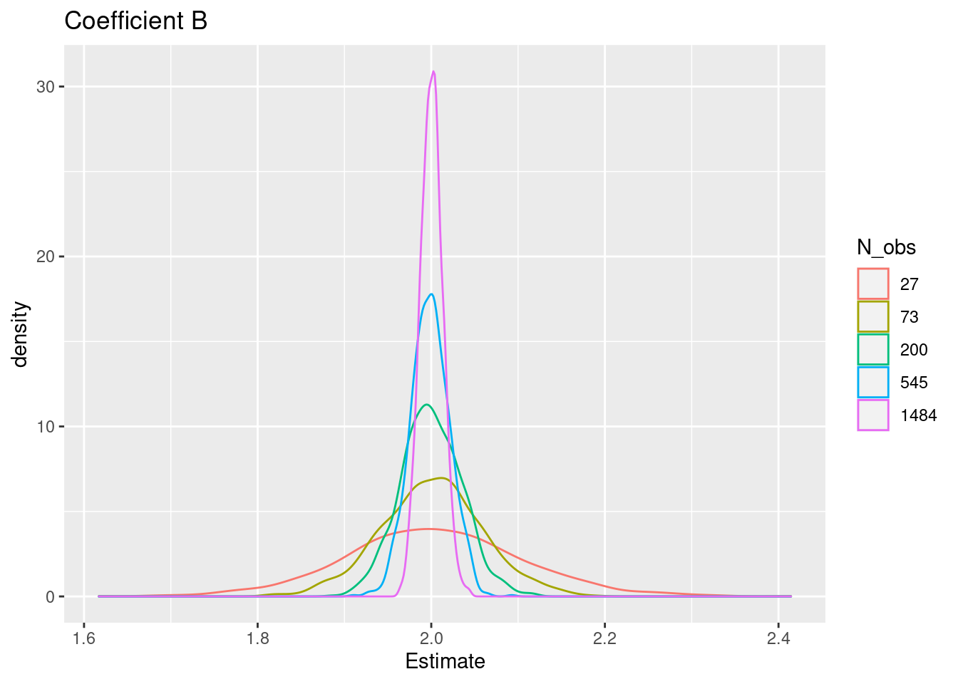
- Test the relationship between sample size and estimation error
ntest <- 1000
coeffA <- matrix(NA, nrow=ntest, ncol=5)
coeffB <- matrix(NA, nrow=ntest, ncol=5)
for (j in c(1:5)) {
    for (i in c(1:ntest)) {
        ns <- floor(10*exp(j))
        x1 <- rnorm(ns, 0, 1)
        x2 <- rnorm(ns, 0, 2)
        y <- 1 + 0.5*x1 + 2*x2 + rnorm(ns, 0, 1)
        mod <- lm(y ~ x1 + x2)
        coeffA[i,j] <- mod$coefficients[2]
        coeffB[i,j] <- mod$coefficients[3]
    }
}
coeffA <- as.data.frame(coeffA)
coeffB <- as.data.frame(coeffB)
names(coeffB) <- names(coeffA) <- as.character(floor(10*exp(c(1:5))))
head(coeffA)
##          27        73       200       545      1484
## 1 0.5612132 0.5519929 0.5477767 0.5050881 0.5242226
## 2 0.5809357 0.6579468 0.6327897 0.5287777 0.4673312
## 3 0.5166434 0.5079282 0.5569459 0.4790036 0.5275614
## 4 0.7021141 0.7058737 0.5240559 0.4516902 0.5161326
## 5 0.4747378 0.5693699 0.5334680 0.4593847 0.4818484
## 6 0.2278944 0.4983064 0.5258636 0.4840685 0.4753997
coeffAA <- melt(coeffA, id.vars=0, variable.name = "N_obs", value.name = "Estimate")
## Warning in melt(coeffA, id.vars = 0, variable.name = "N_obs", value.name =
## "Estimate"): The melt generic in data.table has been passed a data.frame and
## will attempt to redirect to the relevant reshape2 method; please note that
## reshape2 is deprecated, and this redirection is now deprecated as well. To
## continue using melt methods from reshape2 while both libraries are attached,
## e.g. melt.list, you can prepend the namespace like reshape2::melt(coeffA). In
## the next version, this warning will become an error.
head(coeffAA)
##   N_obs  Estimate
## 1    27 0.5612132
## 2    27 0.5809357
## 3    27 0.5166434
## 4    27 0.7021141
## 5    27 0.4747378
## 6    27 0.2278944
coeffBB <- melt(coeffB, id.vars=0, variable.name = "N_obs", value.name = "Estimate")
## Warning in melt(coeffB, id.vars = 0, variable.name = "N_obs", value.name =
## "Estimate"): The melt generic in data.table has been passed a data.frame and
## will attempt to redirect to the relevant reshape2 method; please note that
## reshape2 is deprecated, and this redirection is now deprecated as well. To
## continue using melt methods from reshape2 while both libraries are attached,
## e.g. melt.list, you can prepend the namespace like reshape2::melt(coeffB). In
## the next version, this warning will become an error.
ggplot(coeffAA, aes(x=Estimate, group=N_obs, color=N_obs)) + geom_density() +
    ggtitle("Coefficient A")

ggplot(coeffBB, aes(x=Estimate, group=N_obs, color=N_obs)) + geom_density() +
    ggtitle("Coefficient B")