Data structures
Data types
- Vectors: A single column of data (even a column of length 1)
- Matrices: Two-dimensiona data (all rows and columns of all the same type)
- Arrays: Multi-dimensional data (all rows and columns of all the same type)
- Dataframes: Similar to matrics, but the columns can have different data types
- Dataframes are the most common data structure in R
- Datatables: Similar to dataframes but uses a different syntax
- Lists: are arbitrary combinations of disparate object types in R
Indexing in dataframes
- Rows, columns, and cells in a dataframe is accessed through indexing
df <- data.frame(a = c(1,2,3,4,5), b=c(4, 3, 6, 1, 1), c=c("a", "a", "b", "c", "c"))
# A column
df[, 3]
## [1] "a" "a" "b" "c" "c"
df[,"c"]
## [1] "a" "a" "b" "c" "c"
df$c
## [1] "a" "a" "b" "c" "c"
# Single cell
df[2,3]
## [1] "a"
df$c[2]
## [1] "a"
# A row
df[2,]
##   a b c
## 2 2 3 a
# A range
df[3:5, 2:3]
##   b c
## 3 6 b
## 4 1 c
## 5 1 c
# By name
df[3:4, "c"]
## [1] "b" "c"
# Combining two dataframes
dc <- data.frame(d = c(10,20,30,40,50), e=c("a1", "a2", "b3", "d3", "e2"))
dr <- c(100,200,300,400, 500)
# Column append
df
##   a b c
## 1 1 4 a
## 2 2 3 a
## 3 3 6 b
## 4 4 1 c
## 5 5 1 c
df <- cbind(df, dc)
df
##   a b c  d  e
## 1 1 4 a 10 a1
## 2 2 3 a 20 a2
## 3 3 6 b 30 b3
## 4 4 1 c 40 d3
## 5 5 1 c 50 e2
# Row append
df <- rbind(df, dr)
df
##     a   b   c   d   e
## 1   1   4   a  10  a1
## 2   2   3   a  20  a2
## 3   3   6   b  30  b3
## 4   4   1   c  40  d3
## 5   5   1   c  50  e2
## 6 100 200 300 400 500
# Notice the missing values!!
Data entry
Manual data entry
dt <- data.frame(a = c(1:10), b = rnorm(10, 0, 0.5), c = c(1:2))
dt$d <- dt$a + dt$b + 2*dt$c
dt <- within(dt, e <- a + b + 2*c)
dt
##     a           b c         d         e
## 1   1 -0.21263369 1  2.787366  2.787366
## 2   2 -0.66247029 2  5.337530  5.337530
## 3   3  0.48668178 1  5.486682  5.486682
## 4   4  0.67127390 2  8.671274  8.671274
## 5   5  0.07837078 1  7.078371  7.078371
## 6   6  0.06481947 2 10.064819 10.064819
## 7   7 -0.06772844 1  8.932272  8.932272
## 8   8  0.37295705 2 12.372957 12.372957
## 9   9 -0.25040260 1 10.749597 10.749597
## 10 10  0.56363371 2 14.563634 14.563634
a <- c(1, 2, 4, 2, 6, 3, 5, 8, 1, 10)
b <- rep(c(2:3), times=5)
c <- rep(c(2:3), each=5)
d <- rep(c(2:3), length.out=10)
e <- seq(0, 180, length.out = 10)
f <- seq(0, 45, by=5)
dd <- data.frame(a, b, c, d, e, f)
dd
##     a b c d   e  f
## 1   1 2 2 2   0  0
## 2   2 3 2 3  20  5
## 3   4 2 2 2  40 10
## 4   2 3 2 3  60 15
## 5   6 2 2 2  80 20
## 6   3 3 3 3 100 25
## 7   5 2 3 2 120 30
## 8   8 3 3 3 140 35
## 9   1 2 3 2 160 40
## 10 10 3 3 3 180 45
Empty data.frame
dt <- data.frame(a = character(), b = integer(), c = double())
dt
## [1] a b c
## <0 rows> (or 0-length row.names)
summary(dt)
##       a                   b             c
##  Length:0           Min.   : NA   Min.   : NA
##  Class :character   1st Qu.: NA   1st Qu.: NA
##  Mode  :character   Median : NA   Median : NA
##                     Mean   :NaN   Mean   :NaN
##                     3rd Qu.: NA   3rd Qu.: NA
##                     Max.   : NA   Max.   : NA
Read from the clipboard
- This is not a good practice! Don’t do it.
dt <- read.table(file = "clipboard", header = TRUE)
dt <- data.frame(a = c(1:10), b = rnorm(10, 0, 0.5), c = c(1:2))
write.table(dt, file="clipboard")
write.csv(dt, file="dtdata.csv")
Read from a csv file
data.csv <- read.csv("filename", header = TRUE)
data.csv <- read.csv("URLaddress", header = TRUE)
* Decimal point
* Seperator
* Quotes for strings
* Dates
* Strings as factors (stringAsFactors = FALSE)
View the data
- RStudio “Environment” pane
- Structure of the data
dt <- data.frame(a = c(1:1000), b = rnorm(1000, 0, 1),
    c = c(1:2), d = sample(5, 1000, replace = TRUE))
dt$b[runif(100)<0.1] <- NA
dt$d[runif(100)<0.1] <- NA
dt <- within(dt, e <- c + (c-1)*d  + (b * (c-1) * (d/5)) + rnorm(1000, 0, 1))
head(dt)
##   a           b c  d          e
## 1 1  0.22907528 1  1 -0.8338923
## 2 2 -0.30562656 2  1  1.7661081
## 3 3 -0.22682121 1  5  2.5117719
## 4 4 -0.92552389 2  1  2.1373351
## 5 5 -2.16848987 1  2  0.8061105
## 6 6  0.06662763 2 NA         NA
tail(dt)
##         a          b c  d         e
## 995   995 -0.1063338 1  2  1.029691
## 996   996  1.8169383 2  5 10.144189
## 997   997  0.1109028 1  5  1.671632
## 998   998  1.1378945 2  4  7.011094
## 999   999  0.3246252 1 NA        NA
## 1000 1000 -0.5191283 2  1  2.311693
colnames(dt)
## [1] "a" "b" "c" "d" "e"
dim(dt)
## [1] 1000 5
str(dt)
## 'data.frame':    1000 obs. of  5 variables:
##  $ a: int  1 2 3 4 5 6 7 8 9 10 ...
##  $ b: num  0.229 -0.306 -0.227 -0.926 -2.168 ...
##  $ c: int  1 2 1 2 1 2 1 2 1 2 ...
##  $ d: int  1 1 5 1 2 NA 5 3 4 5 ...
##  $ e: num  -0.834 1.766 2.512 2.137 0.806 ...
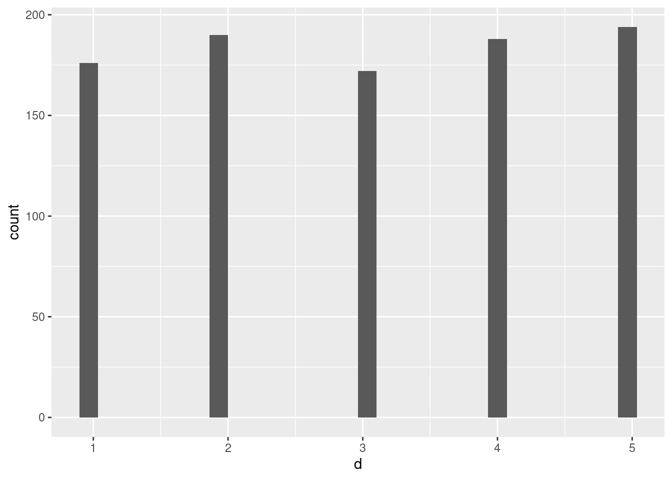
table(dt$d)
##
##   1   2   3   4   5
## 176 190 172 188 194
table(dt$c, dt$d)
##
##      1  2  3  4  5
##   1 80 97 85 89 99
##   2 96 93 87 99 95
xtabs( ~ c + d, data = dt)
##    d
## c    1  2  3  4  5
##   1 80 97 85 89 99
##   2 96 93 87 99 95
Data preparation
Missing values
library(mice)
# Check the pattern of missing data
md.pattern(dt)

##     a c  b  d   e
## 860 1 1  1  1   1   0
## 80  1 1  1  0   0   2
## 60  1 1  0  1   0   2
##     0 0 60 80 140 280
Descriptive statistics
summary(dt)
##        a                b                  c             d
##  Min.   :   1.0   Min.   :-3.38603   Min.   :1.0   Min.   :1.000
##  1st Qu.: 250.8   1st Qu.:-0.68352   1st Qu.:1.0   1st Qu.:2.000
##  Median : 500.5   Median :-0.00996   Median :1.5   Median :3.000
##  Mean   : 500.5   Mean   : 0.01460   Mean   :1.5   Mean   :3.037
##  3rd Qu.: 750.2   3rd Qu.: 0.70750   3rd Qu.:2.0   3rd Qu.:4.000
##  Max.   :1000.0   Max.   : 2.91005   Max.   :2.0   Max.   :5.000
##                   NA's   :60                       NA's   :80
##        e
##  Min.   :-2.6710
##  1st Qu.: 0.9593
##  Median : 2.5593
##  Mean   : 3.0548
##  3rd Qu.: 4.9061
##  Max.   :10.1442
##  NA's   :140
summary(subset(dt, c == 1))
##        a               b                  c           d
##  Min.   :  1.0   Min.   :-3.38603   Min.   :1   Min.   :1.000
##  1st Qu.:250.5   1st Qu.:-0.54220   1st Qu.:1   1st Qu.:2.000
##  Median :500.0   Median : 0.08055   Median :1   Median :3.000
##  Mean   :500.0   Mean   : 0.08491   Mean   :1   Mean   :3.067
##  3rd Qu.:749.5   3rd Qu.: 0.78316   3rd Qu.:1   3rd Qu.:4.000
##  Max.   :999.0   Max.   : 2.91005   Max.   :1   Max.   :5.000
##                  NA's   :50                     NA's   :50
##        e
##  Min.   :-2.6710
##  1st Qu.: 0.2744
##  Median : 0.8979
##  Mean   : 0.8894
##  3rd Qu.: 1.5399
##  Max.   : 3.7475
##  NA's   :100
summary(subset(dt, c == 2))
##        a                b                  c           d
##  Min.   :   2.0   Min.   :-2.90016   Min.   :2   Min.   :1.000
##  1st Qu.: 251.5   1st Qu.:-0.74860   1st Qu.:2   1st Qu.:2.000
##  Median : 501.0   Median :-0.07744   Median :2   Median :3.000
##  Mean   : 501.0   Mean   :-0.04997   Mean   :2   Mean   :3.009
##  3rd Qu.: 750.5   3rd Qu.: 0.65761   3rd Qu.:2   3rd Qu.:4.000
##  Max.   :1000.0   Max.   : 2.49612   Max.   :2   Max.   :5.000
##                   NA's   :10                     NA's   :30
##        e
##  Min.   : 0.9236
##  1st Qu.: 3.5177
##  Median : 4.7754
##  Mean   : 4.9378
##  3rd Qu.: 6.3294
##  Max.   :10.1442
##  NA's   :40
library(stargazer)
stargazer(dt, type="html", digits = 1)
|
|
|
Statistic
|
N
|
Mean
|
St. Dev.
|
Min
|
Pctl(25)
|
Pctl(75)
|
Max
|
|
|
|
a
|
1,000
|
500.5
|
288.8
|
1
|
250.8
|
750.2
|
1,000
|
|
b
|
940
|
0.01
|
1.0
|
-3.4
|
-0.7
|
0.7
|
2.9
|
|
c
|
1,000
|
1.5
|
0.5
|
1
|
1
|
2
|
2
|
|
d
|
920
|
3.0
|
1.4
|
1.0
|
2.0
|
4.0
|
5.0
|
|
e
|
860
|
3.1
|
2.5
|
-2.7
|
1.0
|
4.9
|
10.1
|
|
|
Plots
library(ggplot2)
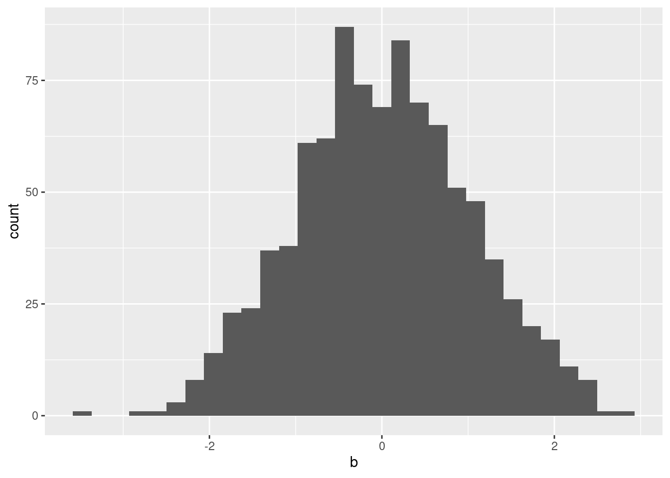
ggplot(dt, aes(x = b)) + geom_histogram()
## `stat_bin()` using `bins = 30`. Pick better value with `binwidth`.
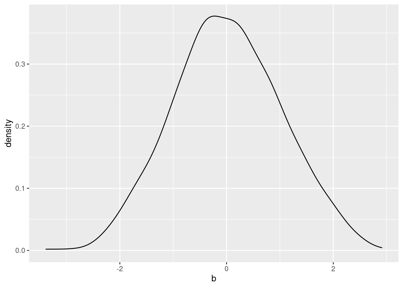
ggplot(dt, aes(x = b)) + geom_density()
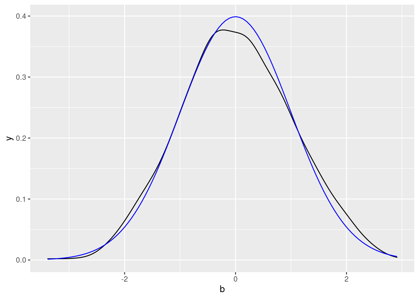
ggplot(dt, aes(x = b)) + geom_density() +
 stat_function(fun = dnorm, args = list(mean = 0, sd = 1), col="blue")
ggplot(dt, aes(x = d)) + geom_histogram()
## `stat_bin()` using `bins = 30`. Pick better value with `binwidth`.
ggplot(dt, aes(x = d)) + geom_histogram(binwidth=1)
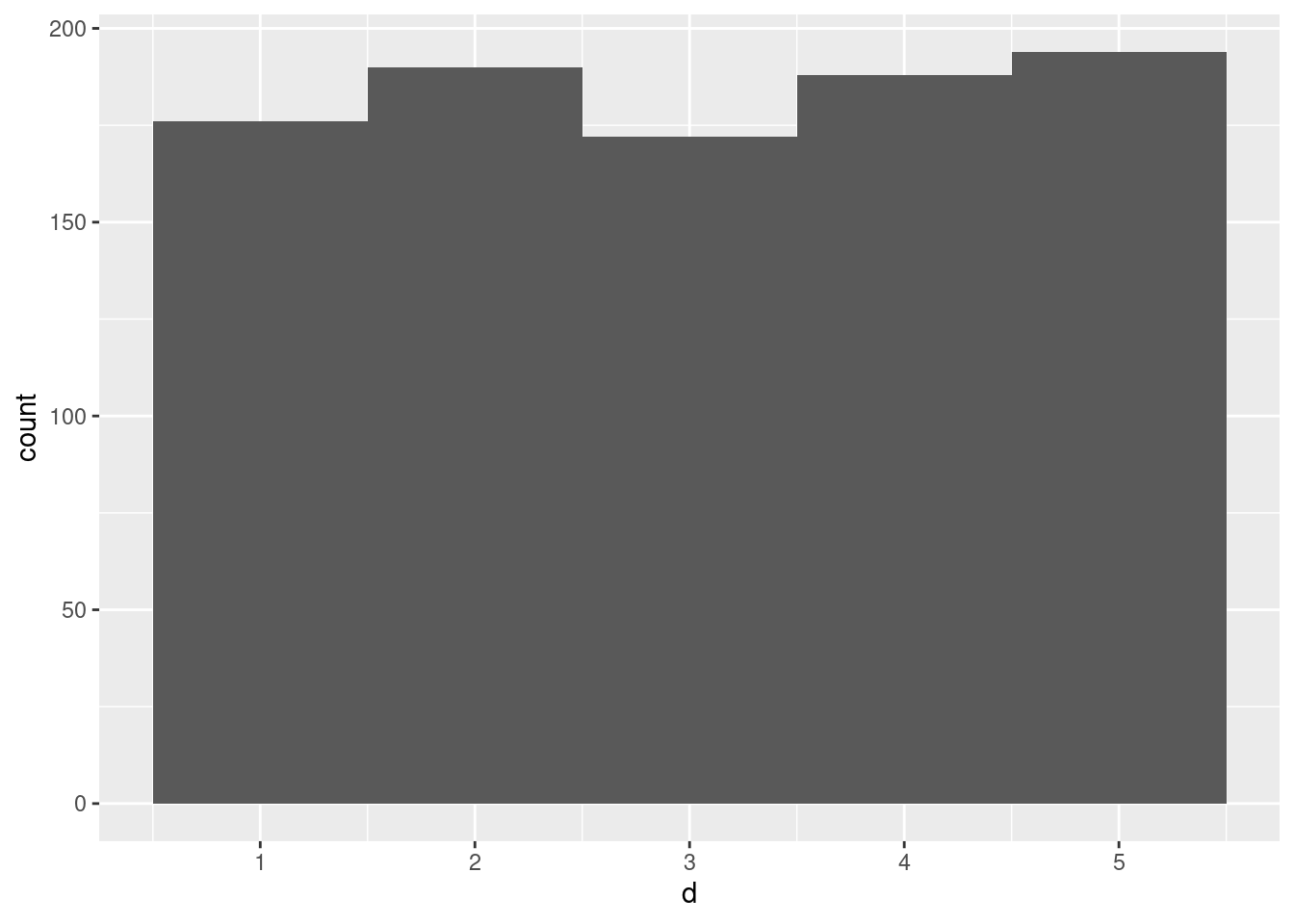
ggplot(dt, aes(x = d)) + geom_bar()

ggplot(dt, aes(x = d, y = b)) + geom_point()

ggplot(dt, aes(x = d, y = b)) + geom_point(size=5)
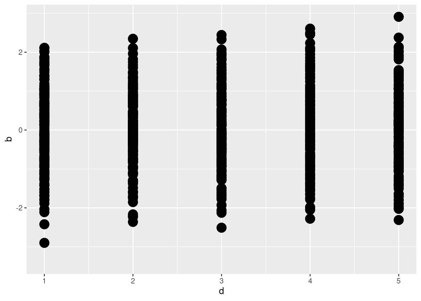
ggplot(dt, aes(x = d, y = b)) + geom_point(size=5, alpha=0.1)
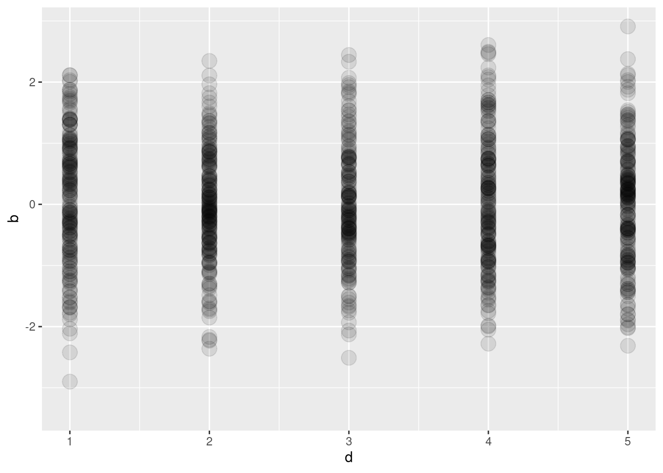
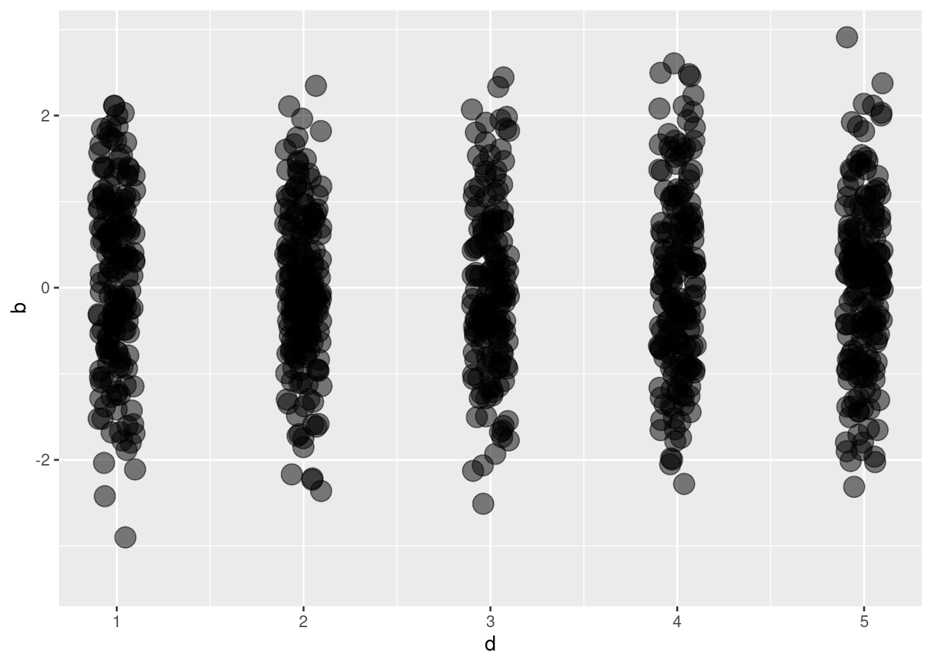
# If overplotted...
ggplot(dt, aes(x = d, y = b)) + geom_jitter(size=5, alpha=0.5, width=0.1)
ggplot(dt, aes(x = d, y = b)) + geom_jitter(size=5, alpha=0.5, width=0.5)

# Bivariate plots
ggplot(dt, aes(x = b, y = e)) + geom_point()

ggplot(dt, aes(x = b, y = e)) + geom_point() +
    geom_smooth(formula = y ~ x)
## `geom_smooth()` using method = 'gam'
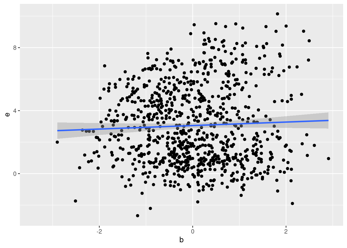
ggplot(dt, aes(x = b, y = e)) + geom_point() +
    geom_smooth(formula = y ~ x, se = FALSE, method = "lm")

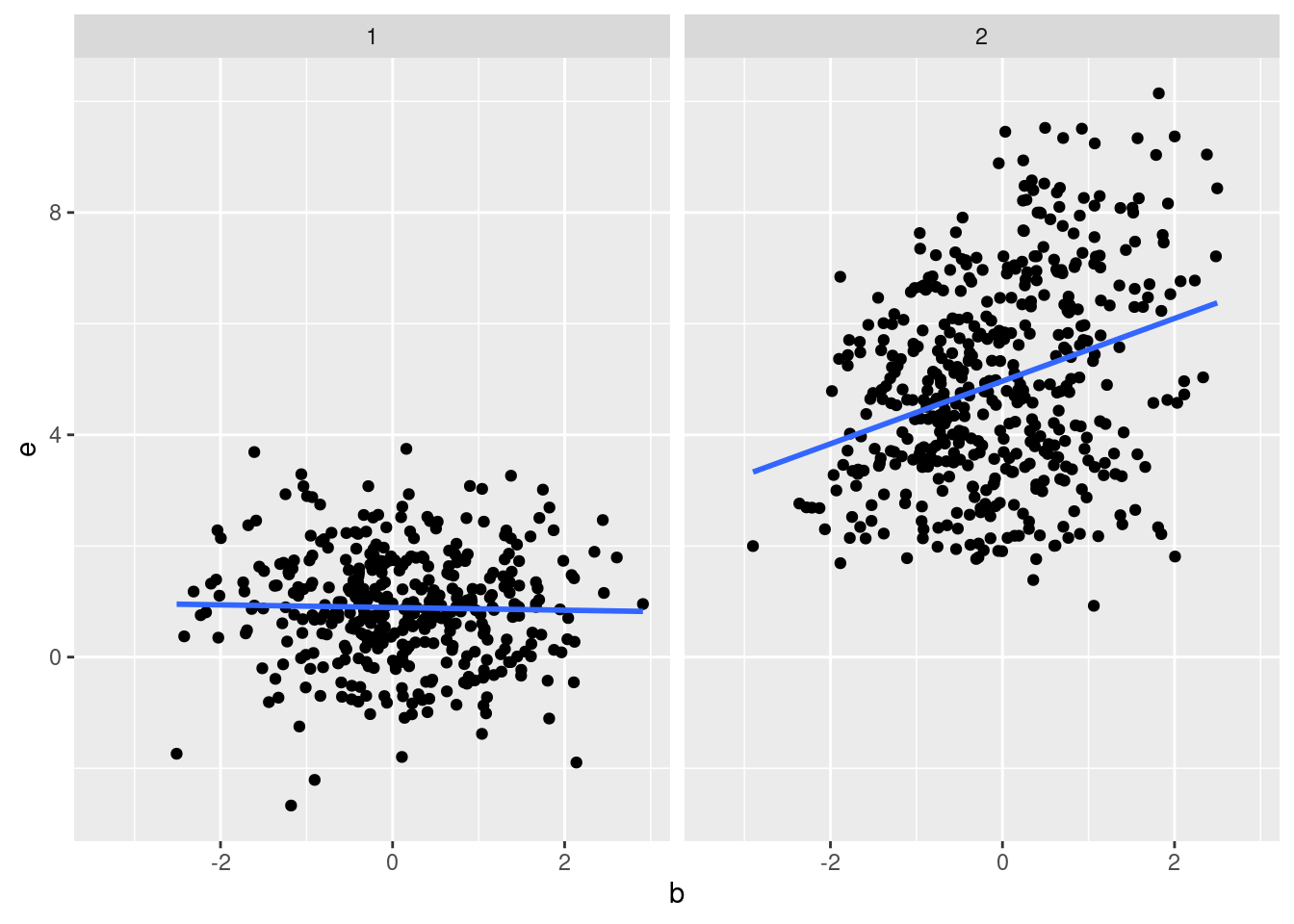
ggplot(dt, aes(x = b, y = e)) + geom_point() + facet_wrap(~ c) +
    geom_smooth(formula = y ~ x, se = FALSE, method = "lm")
ggplot(dt, aes(x = b, y = e)) + geom_point() + facet_wrap(c ~ d, nrow = 2) +
    geom_smooth(formula = y ~ x, se = FALSE, method = "lm")

Correlations
# Correlations - variables 2-4
cor(dt[, 2:5])
##    b  c  d  e
## b  1 NA NA NA
## c NA  1 NA NA
## d NA NA  1 NA
## e NA NA NA  1
cor(dt[, 2:5], use = "complete.obs")
##              b            c            d          e
## b  1.000000000 -0.087614820 -0.006659529 0.04413574
## c -0.087614820  1.000000000 -0.008355224 0.79864265
## d -0.006659529 -0.008355224  1.000000000 0.28556941
## e  0.044135737  0.798642651  0.285569414 1.00000000
cor(dt[, 2:5], use = "pairwise.complete.obs")
##              b           c            d          e
## b  1.000000000 -0.06675139 -0.006659529 0.04413574
## c -0.066751395  1.00000000 -0.020463507 0.79864265
## d -0.006659529 -0.02046351  1.000000000 0.28556941
## e  0.044135737  0.79864265  0.285569414 1.00000000
cor(dt[, 2:5], use = "pairwise.complete.obs", method = "kendall")
##              b           c           d            e
## b  1.000000000 -0.05573957 -0.01208753 -0.004163847
## c -0.055739569  1.00000000 -0.01848081  0.684466967
## d -0.012087530 -0.01848081  1.00000000  0.175086125
## e -0.004163847  0.68446697  0.17508613  1.000000000
cor(dt[, 2:5], use = "pairwise.complete.obs", method = "spearman")
##              b           c           d            e
## b  1.000000000 -0.06823047 -0.01555521 -0.008163688
## c -0.068230469  1.00000000 -0.02065941  0.837810450
## d -0.015555208 -0.02065941  1.00000000  0.218904443
## e -0.008163688  0.83781045  0.21890444  1.000000000
Plot all data all together
library(GGally)
ggpairs(dt)
## plot: [1,1] [=>------------------------------------------------] 4% est: 0s
## plot: [1,2] [===>----------------------------------------------] 8% est: 1s
## plot: [1,3] [=====>--------------------------------------------] 12% est: 1s
## plot: [1,4] [=======>------------------------------------------] 16% est: 1s
## plot: [1,5] [=========>----------------------------------------] 20% est: 1s
## plot: [2,1] [===========>--------------------------------------] 24% est: 1s
## plot: [2,2] [=============>------------------------------------] 28% est: 1s
## plot: [2,3] [===============>----------------------------------] 32% est: 1s
## plot: [2,4] [=================>--------------------------------] 36% est: 1s
## plot: [2,5] [===================>------------------------------] 40% est: 1s
## plot: [3,1] [=====================>----------------------------] 44% est: 1s
## plot: [3,2] [=======================>--------------------------] 48% est: 1s
## plot: [3,3] [=========================>------------------------] 52% est: 1s
## plot: [3,4] [===========================>----------------------] 56% est: 1s
## plot: [3,5] [=============================>--------------------] 60% est: 1s
## plot: [4,1] [===============================>------------------] 64% est: 0s
## plot: [4,2] [=================================>----------------] 68% est: 0s
## plot: [4,3] [===================================>--------------] 72% est: 0s
## plot: [4,4] [=====================================>------------] 76% est: 0s
## plot: [4,5] [=======================================>----------] 80% est: 0s
## plot: [5,1] [=========================================>--------] 84% est: 0s
## plot: [5,2] [===========================================>------] 88% est: 0s
## plot: [5,3] [=============================================>----] 92% est: 0s
## plot: [5,4] [===============================================>--] 96% est: 0s
## plot: [5,5] [==================================================]100% est: 0s

Basic tests
- Chi-square test for categorical variables
tab <- xtabs(~ c + d, data = dt)
tab
##    d
## c    1  2  3  4  5
##   1 80 97 85 89 99
##   2 96 93 87 99 95
chisq.test(tab)
##
##  Pearson's Chi-squared test
##
## data:  tab
## X-squared = 1.7424, df = 4, p-value = 0.783
- t-test for continuous variables
t.test(dt$b, mu = 0)
##
##  One Sample t-test
##
## data:  dt$b
## t = 0.44309, df = 939, p-value = 0.6578
## alternative hypothesis: true mean is not equal to 0
## 95 percent confidence interval:
##  -0.05005034  0.07924184
## sample estimates:
##  mean of x
## 0.01459575
t.test(dt$b, dt$e)
##
##  Welch Two Sample t-test
##
## data:  dt$b and dt$e
## t = -32.924, df = 1106.3, p-value < 2.2e-16
## alternative hypothesis: true difference in means is not equal to 0
## 95 percent confidence interval:
##  -3.221385 -2.859018
## sample estimates:
##  mean of x  mean of y
## 0.01459575 3.05479695
t.test(dt$b, dt$e, var.equal = TRUE)
##
##  Two Sample t-test
##
## data:  dt$b and dt$e
## t = -34.003, df = 1798, p-value < 2.2e-16
## alternative hypothesis: true difference in means is not equal to 0
## 95 percent confidence interval:
##  -3.215560 -2.864842
## sample estimates:
##  mean of x  mean of y
## 0.01459575 3.05479695
with(dt, t.test(b[c == 1], b[c == 2]))
##
##  Welch Two Sample t-test
##
## data:  b[c == 1] and b[c == 2]
## t = 2.0455, df = 923.58, p-value = 0.04109
## alternative hypothesis: true difference in means is not equal to 0
## 95 percent confidence interval:
##  0.005469478 0.264292485
## sample estimates:
##   mean of x   mean of y
##  0.08490605 -0.04997493
Data visualization
Make a dataset
library(ggplot2)
library(ggthemes)
DT <- data.frame(country = rep(c("A", "B", "C"), each=20), date = rep(1991:2010, times=3),
    gdp = c(1 + cumsum(rnorm(20, 0.01, 0.02)), 1.1 + cumsum(rnorm(20, 0.01, 0.04)),
    1.2 + cumsum(rnorm(20, 0.04, 0.02))))
ggplot graphics
c1 <- ggplot(DT, aes(x=date, y=gdp, color=country)) + geom_line()
c1

# Thick lines
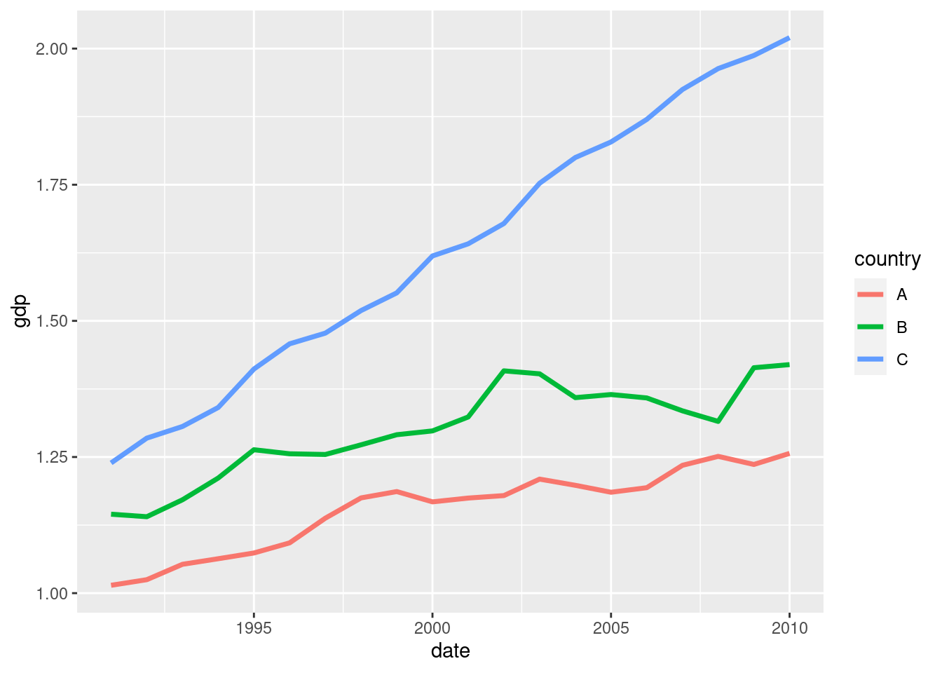
c1 <- ggplot(DT, aes(x=date, y=gdp, color=country)) + geom_line(size=1.25)
c1
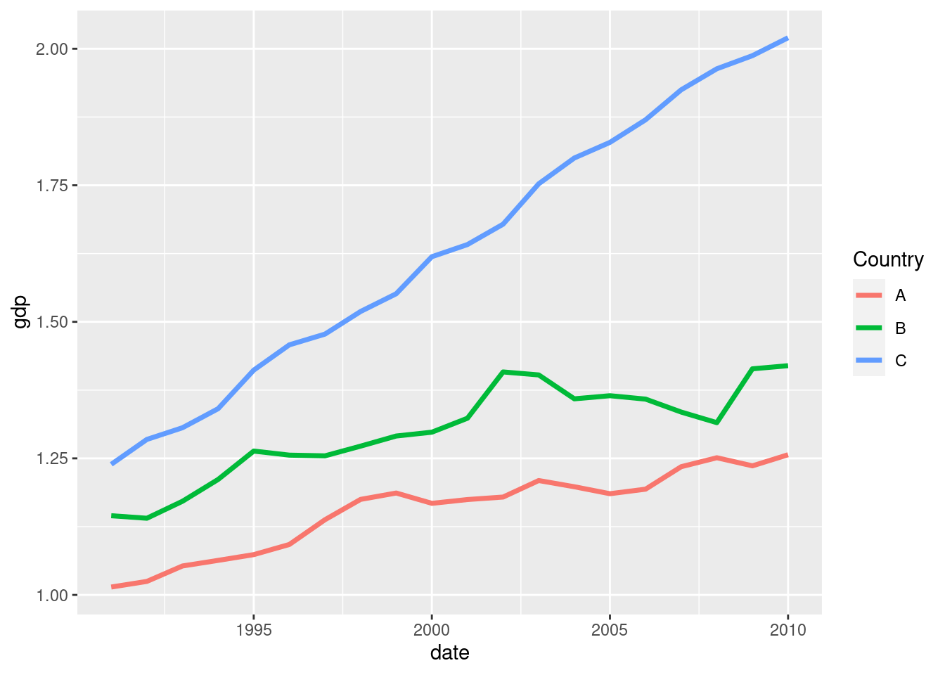
# Change legend title
c1 <- c1 + guides(color = guide_legend(title = "Country"))
c1
# Remove legend text
c1 <- c1 +  guides(color = guide_legend(title = NULL))
c1
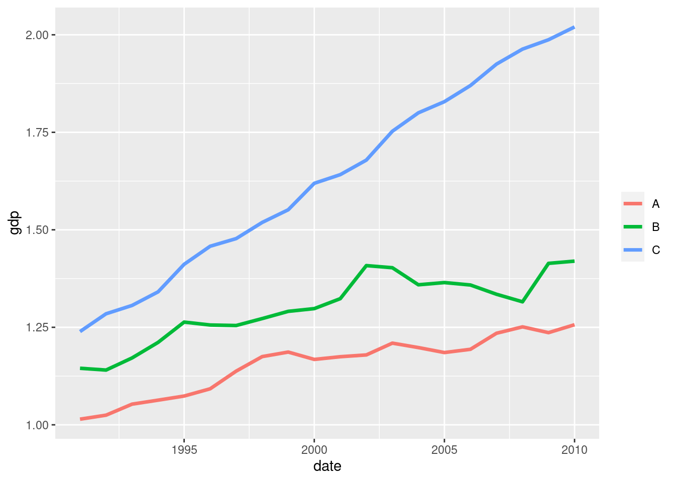
# Add titles
c1 <- c1 + labs(title="GDP level, 1990-2010", x="", y="GDP (Million USD)")
c1
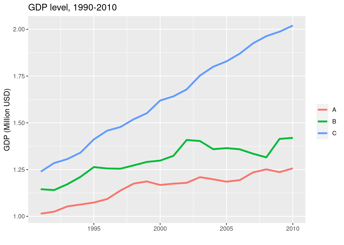
# Bigger title
c1 <- c1 + theme(plot.title = element_text(size = rel(2)))
c1

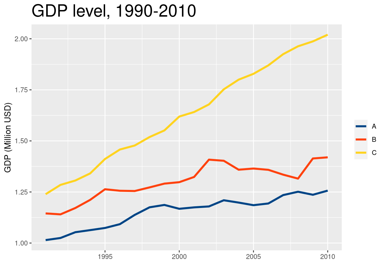
# Use LibreOffice colors
c1 + scale_color_calc()
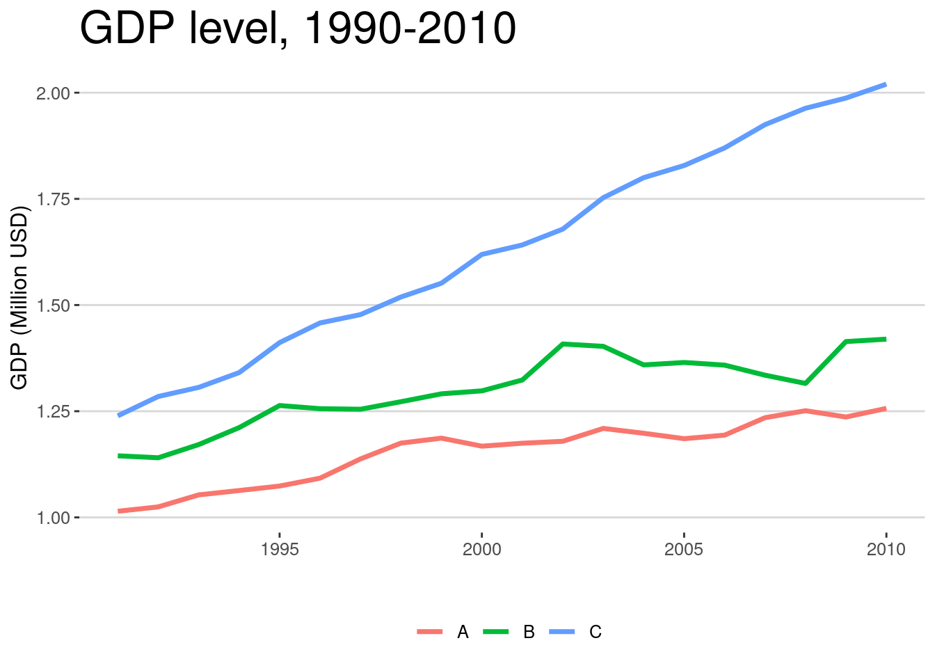
# HC theme
c1 + theme_hc()
# HC theme + axis characteristics
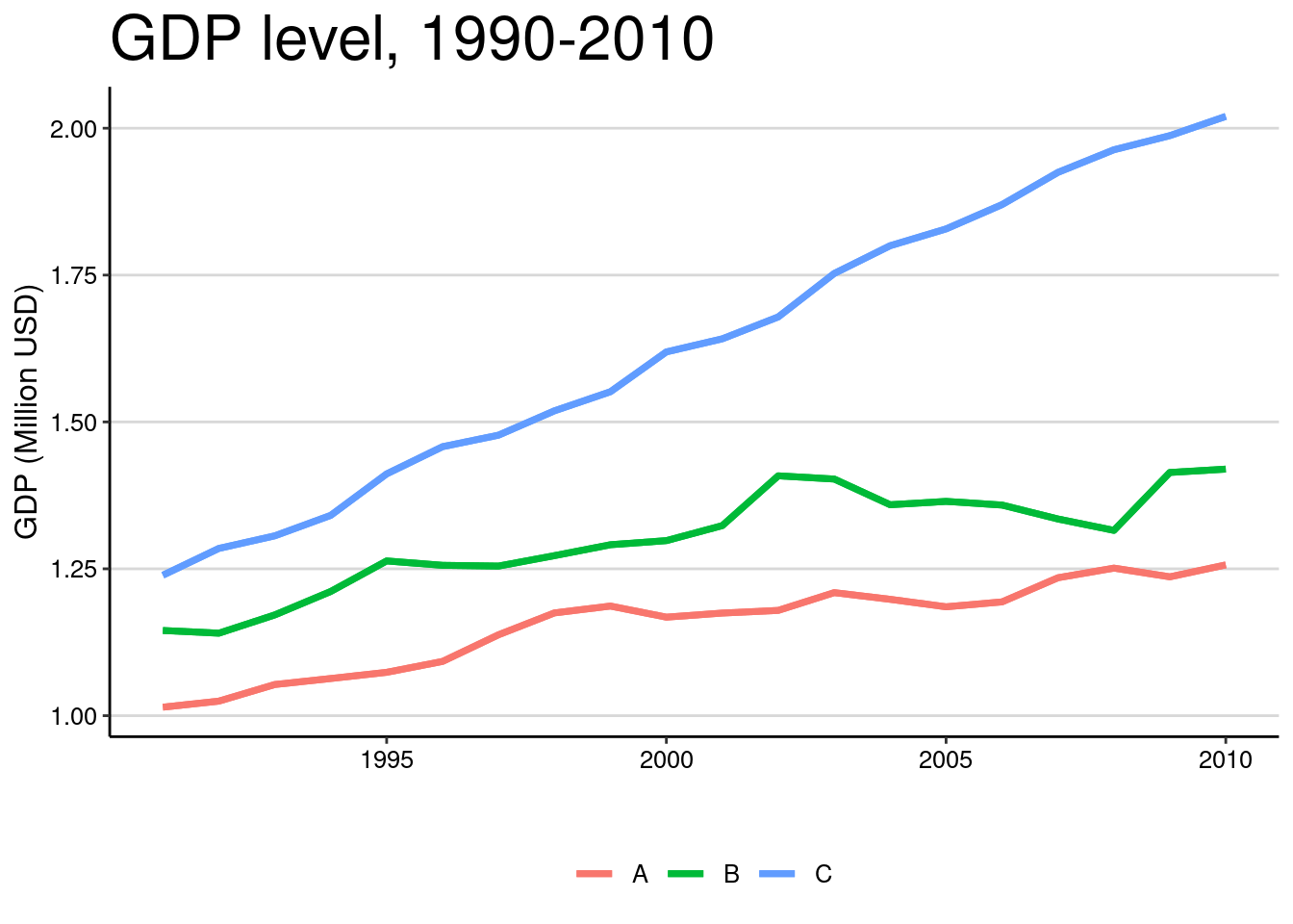
c1 + theme_hc() + theme(axis.line = element_line(colour = "black", size=0.5),
                        axis.text=element_text(colour="black")) + geom_line(size=1.25)
# Classic theme
c1 + theme_classic()

# Minimal  theme
c1 + theme_minimal()

# Economist theme
c1 + theme_economist()

# GoogleDocs theme
c1 + theme_gdocs()

My theme
theme_et <- function (base_size = 12, base_family = "ubuntu") {
  theme(rect = element_rect(fill = "#FFFFFF", linetype = 0, colour = NA),
        text = element_text(size = base_size, family = base_family),
        plot.title = element_text( size = rel(1.1), hjust = 0.5),
        axis.title.x = element_text(hjust = 0.5, size = rel(0.85)),
        axis.title.y = element_text(hjust = 0.5, size = rel(0.85)),
        axis.text = element_text(colour = "black"),
        axis.line = element_line(colour = "black", size = rel(0.3)),
        legend.text = element_text(colour = "black", size= rel(.85)),
        panel.grid.major.y = element_line(color = "gray", size = rel(0.3)),
        panel.grid.major.x = element_blank(),
        panel.grid.minor.y = element_blank(), panel.grid.minor.x = element_blank(),
        panel.border = element_blank(), panel.background = element_blank(),
        legend.position = "bottom", legend.key = element_rect(fill = "#FFFFFF00"))
}

c1 + theme_et()

Modifying themes
c1 + theme(plot.title = element_text(size = rel(2), colour = "blue"))

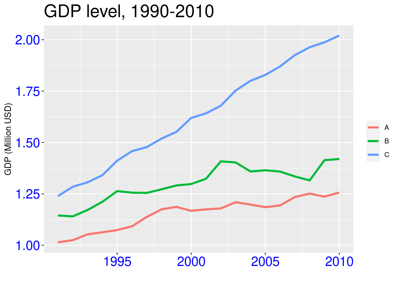
c1 + theme(axis.text = element_text(colour = "blue", size=rel(1.5)))
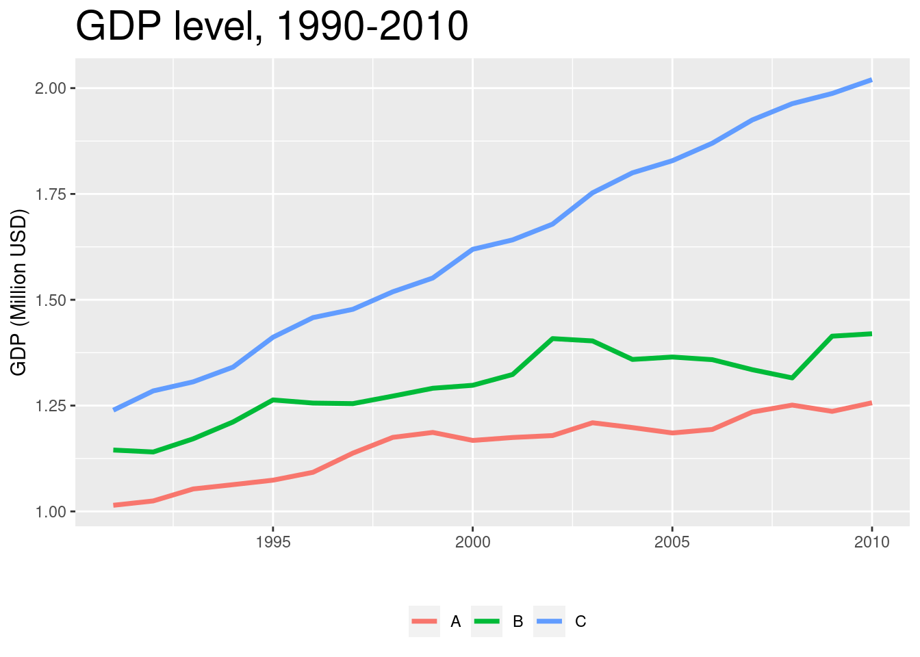
c1 + theme(legend.position = "bottom")
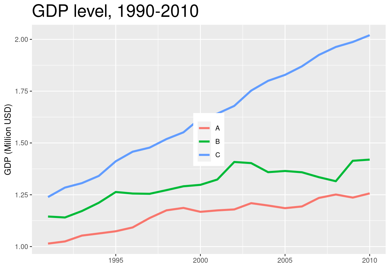
c1 + theme(legend.position = c(0.5, 0.5))
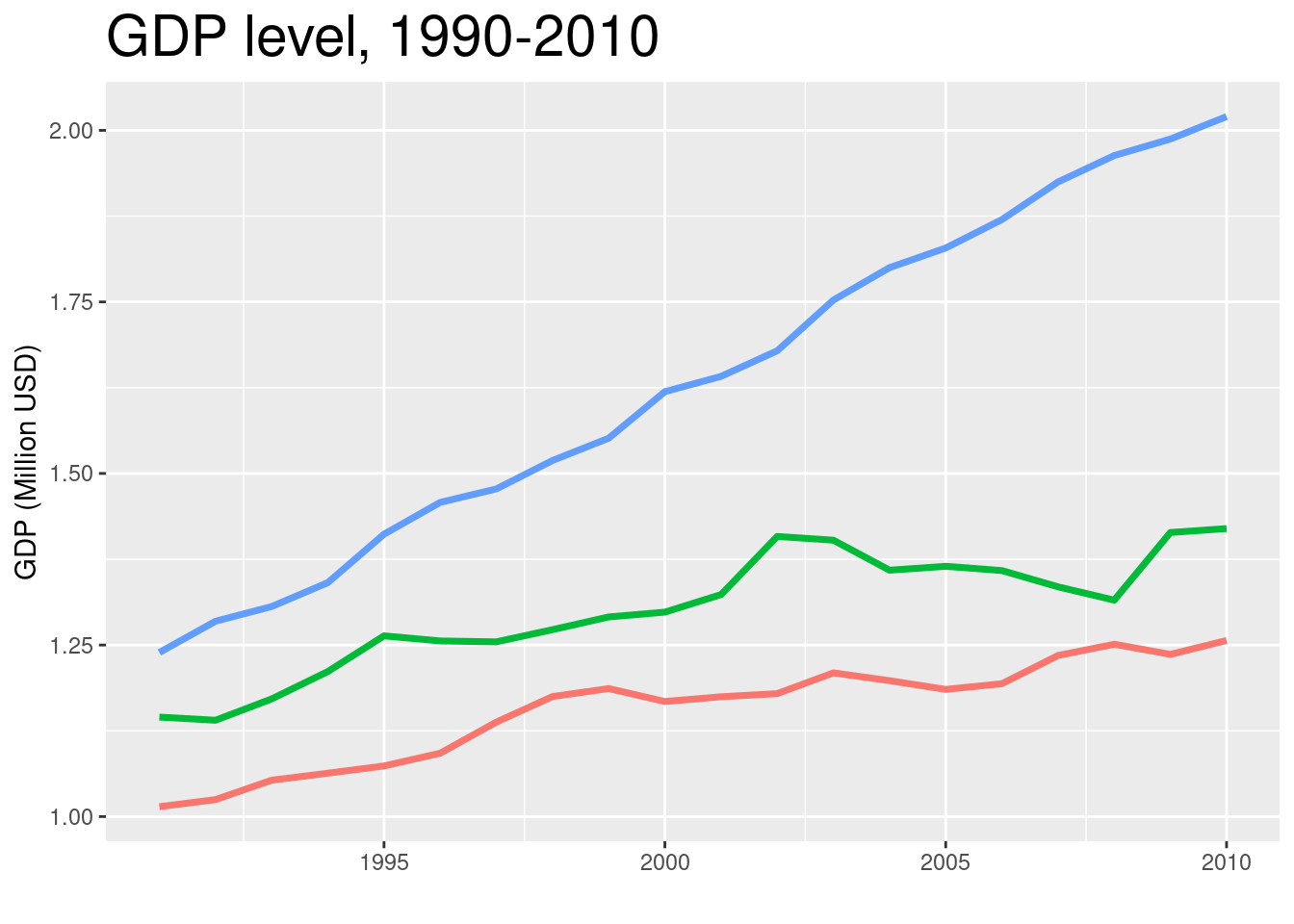
c1 + theme(legend.position = "none")
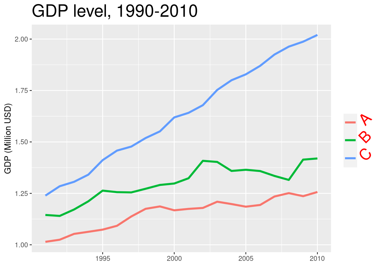
c1 + theme(legend.text = element_text(size = 20, colour = "red", angle = 45))
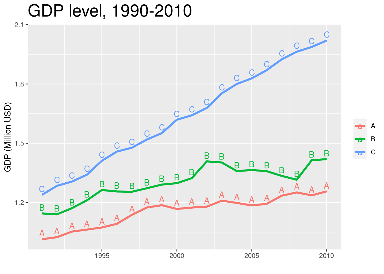
# Add text
c1 + geom_text(data = DT, aes(x=date, y=gdp+.03, label = country))
# Add formula
c1 + annotate("text", x=1995, y=1.5, parse=TRUE, label="frac(1, sqrt(2 * pi)) * e ^ {-x^2 / 2}")
